Notes on Neural Tangent Kernels
Empirical notes on when NTKs work, when assumptions break, and a few explicit kernels on toy models.
NOTE: This is a bunch of notes from studying Neural Tangent Kernels. I wanted to understand empirically what the kernels can be used for and when the assumptions break down. While there is some math, most of it is code on toy models. For those who want to run the code on their own, see this colab
It has explicitly calculated kernels, which may help people if the theory is too abstract.
Why Neural Tangent Kernels?
The functional evolution of a neural network (its outputs on inputs) for MSEloss can be written as a kernel $\Theta_t(x, x_d)$:
\[\frac{df(x)}{dt} = \sum_{x_d}^{\text{train data}} \Theta(x, x_d)\times \big(f(x_d) - y_d\big)\]where we sum over training data $x_d$, using differences between our model $f(x_d)$ and known targets $y_d$.
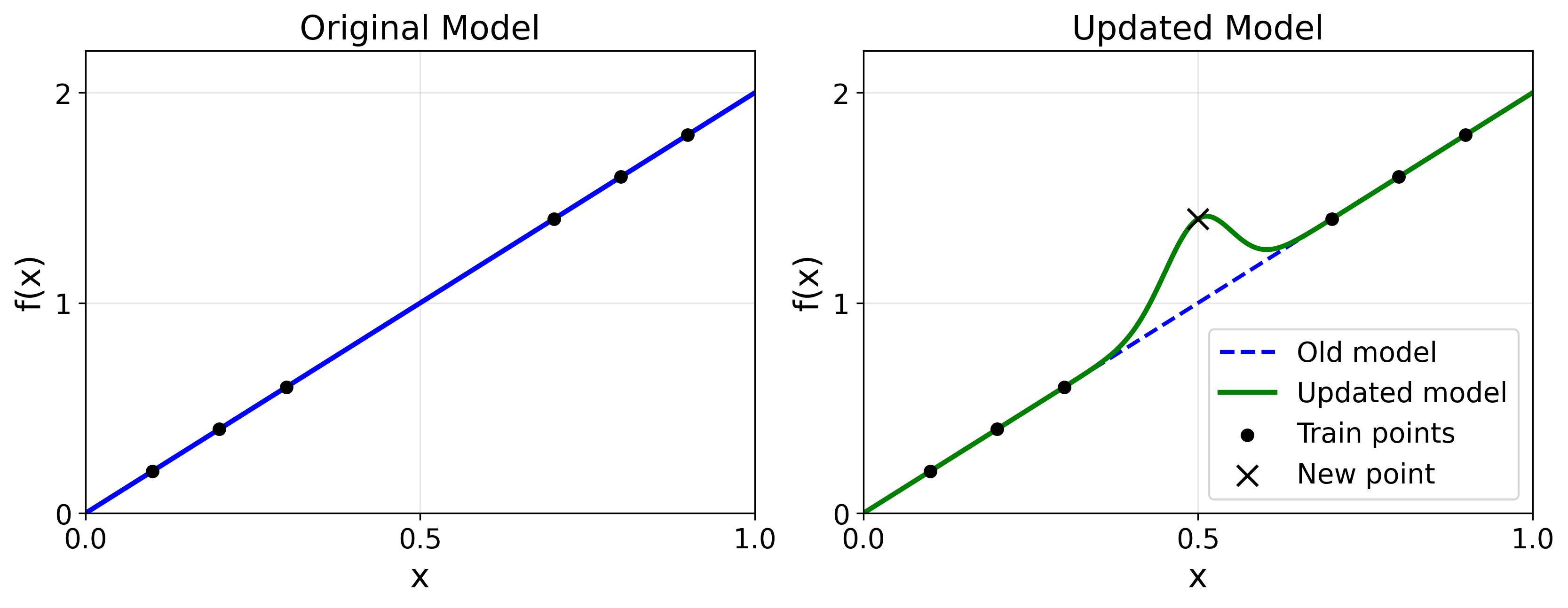
One way to understand this equation: Suppose we’re interested in the value of our function on a point $x$ not in our training data. Fitting our model to the training data will cause its prediction on that point to change, with intuitively the closer points mattering more (e.g., if $(x_d, y_d) = (1,10)$ then a point $x=0.9$ should have a value close to 10). The kernel $\Theta_t(x, x_d)$ captures the “weight” assigned to nearby points in determining the prediction on $x$. This kernel can be computed empirically.
What Is a Kernel?
A kernel is a measure of similarity between points $x_1, x_2$. It is used in kernel regression, where a model guesses the output for an unseen point based off previously seen points. The kernel tells the model which past inputs + outputs are most similar to the current input.
Constant Neural Tangent Kernel
In general this kernel evolves over time - the network will learn features from the data, causing it to change it’s estimate of how different inputs are similar.
But there exists a limit where kernel $\Theta_t$ is constant! This occurs for a certain parameterization (called the NTK parameterization), in the limit of infinitely wide neural networks.
This has several interesting implications:
- The kernel of an infinitely wide neural network is deterministic (no randomness) and can be easily calculated, yielding the time evolution of our network.
- This limit guarantees training finds a global minima for our network.
- The network does not learn features in this limit. Thus it does not describe practical neural networks.
A constant kernel implies linear dynamics, where the gradient does not change direction over training.
That infinite width networks have this property can be proven theoretically, but we can verify it empirically by noting very wide neural networks do not change their weights very much throughout training.
Visualizing Linear Dynamics
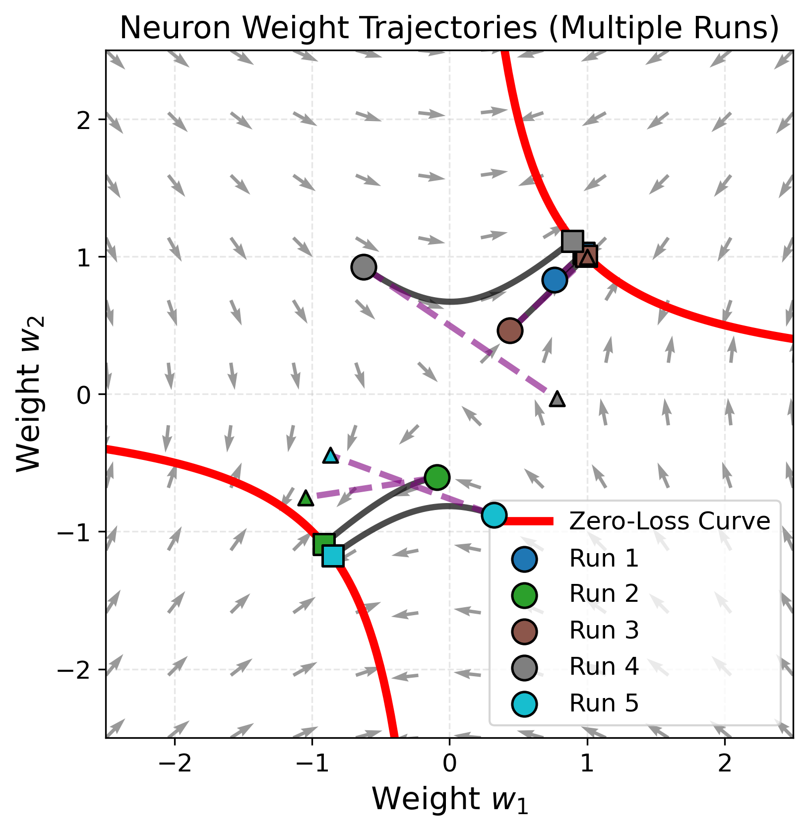
We visualize linear dynamics in a toy model. Consider a network with one hidden layer, with 1D inputs and outputs. Let there be $N$ neurons, each with two weights connected to input and output, $w_{1,i}, w_{2,i}$. The output of a neuron is
\[h_i(x) = w_{2,i}\,\sigma(w_{1,i}x)\]where $\sigma$ is an activation function (e.g., ReLU, a quadratic, or even linear $\sigma(x)=x$). The network prediction on an input $x$ is given by combining all the neurons
\[f(x,\mathbf{w}_1,\mathbf{w}_2)=\sum_{i}^{N} w_{2,i}\,\sigma(w_{1,i}x).\]As further simplification, suppose our training data is a single point $(x,y)=(1,m)$, and our activation function be linear, $\sigma(x)=x$. Fitting the data implies
\[\sum_{i}^{N} w_{2,i}w_{1,i}=m.\]For a single neuron, this implies $w_2=m/w_1$. Since each neuron has only two parameters, the training dynamics can be visualized easily. We also plot a linearized approximation for comparison.
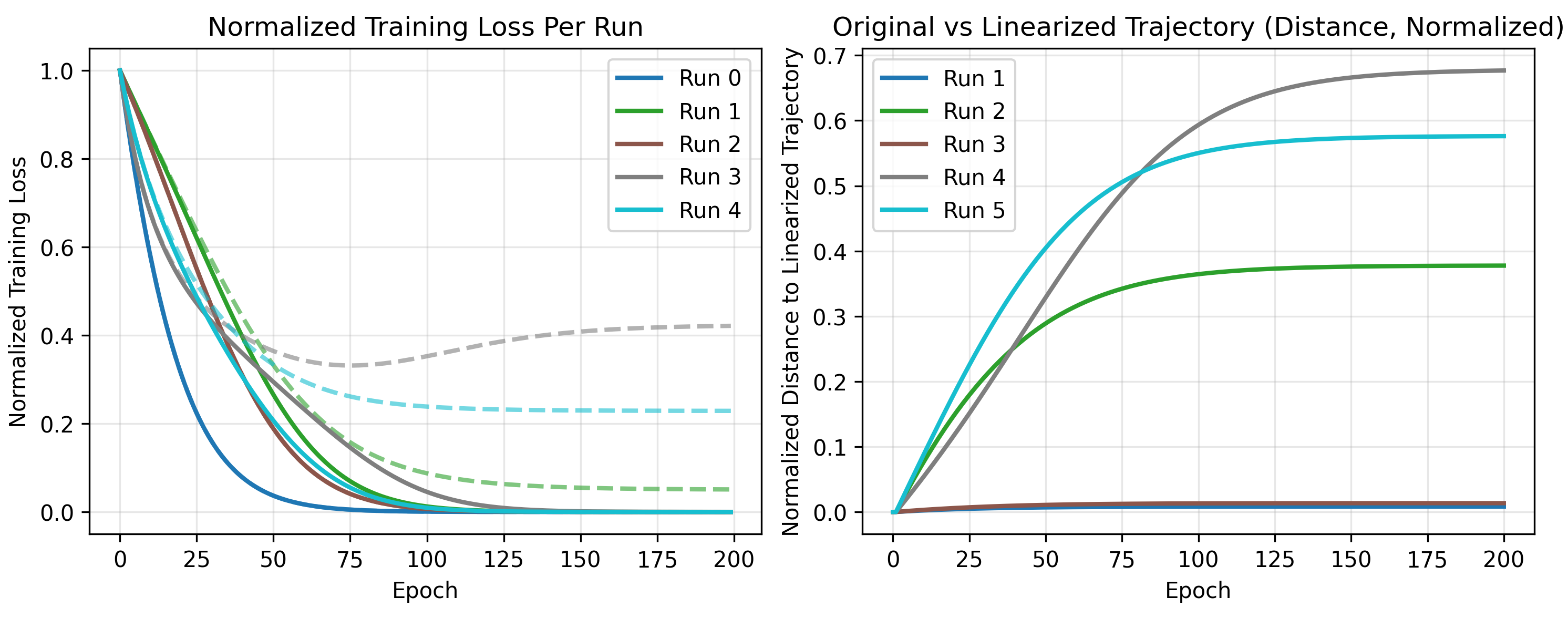
For higher dimensions, this visualization is less useful. As an alternative, we plot the loss along the linearized and actual trajectories, and their differences (in distance in weight space).
Higher Dimensions - More Neurons
One neuron is clearly very nonlinear, but also very far from the infinite width limit.
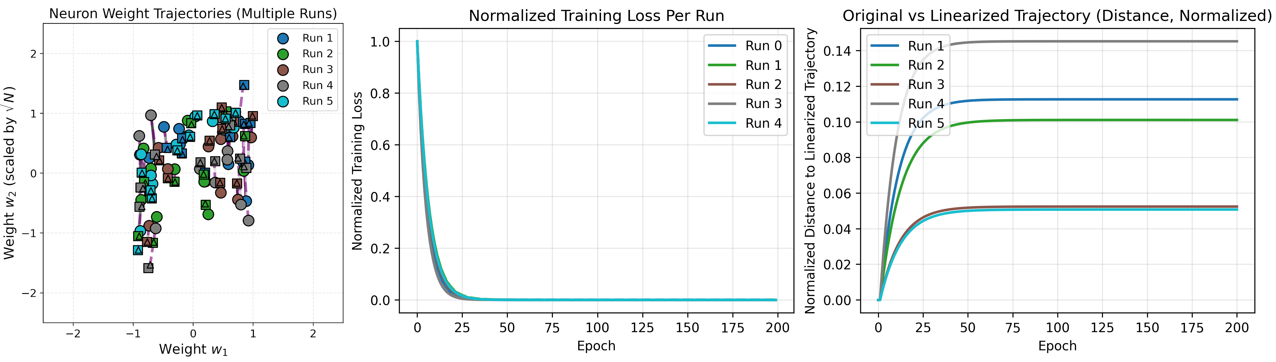
What about two neurons? Note that we follow the standard parameterization here (Kaiming init) where weights are initialized from a uniform distribution sampled from $1/\sqrt{N}$, the dimension of the current layer. To keep weight visualizations interpretable, we rescale the second layer weights, but the rest of the computations are without any rescaling.
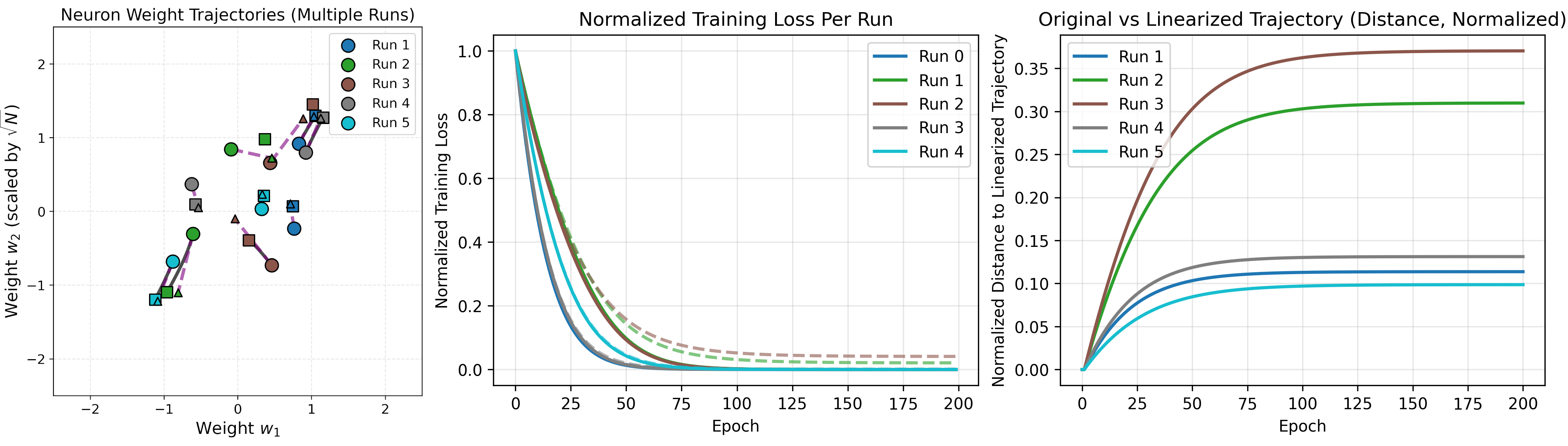
For 10 neurons, there is an even closer match with the linear approximation.
Similarly, 100 neurons:
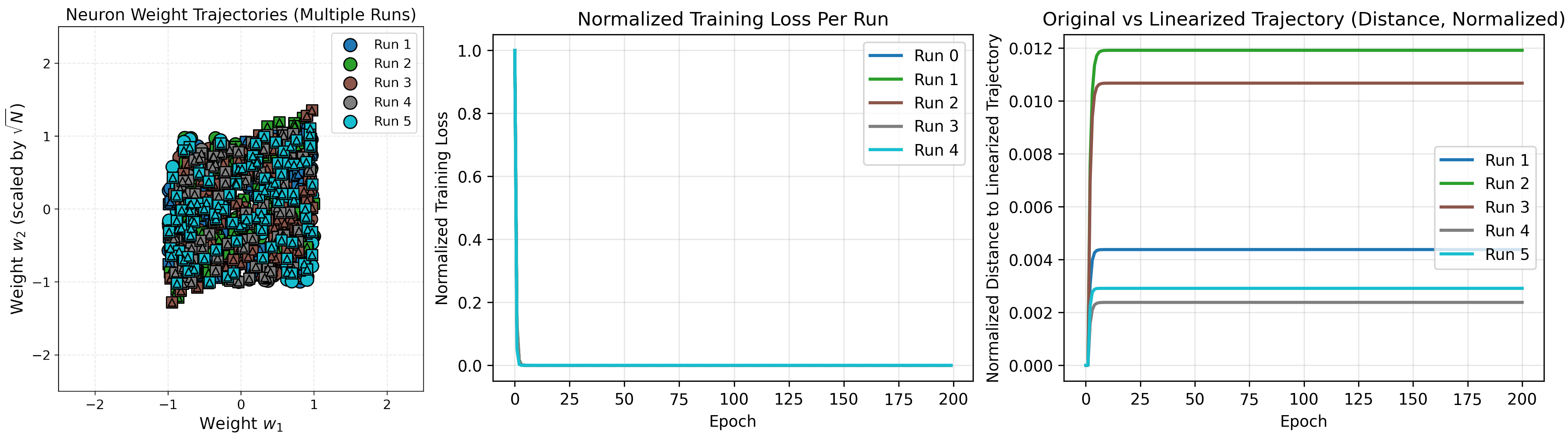
As the number of neurons increase, the error from a linear approximation of training gets smaller (as indicated by the shrinking magnitudes on the right). It also takes increasingly less time to reach an optimum for this network, shown by the loss curves.
At least for this network, we see the infinite width regime is approximately linear.
Are All Infinite Width Networks Linear?
Although we saw wider networks seem closer to valid minima, this does not prove the linear approximation is correct. As a counterargument, one can imagine that more neurons distributes the distance travelled over multiple neurons (reducing the distance per neuron) without changing the nonlinearity, pictured below in the middle.
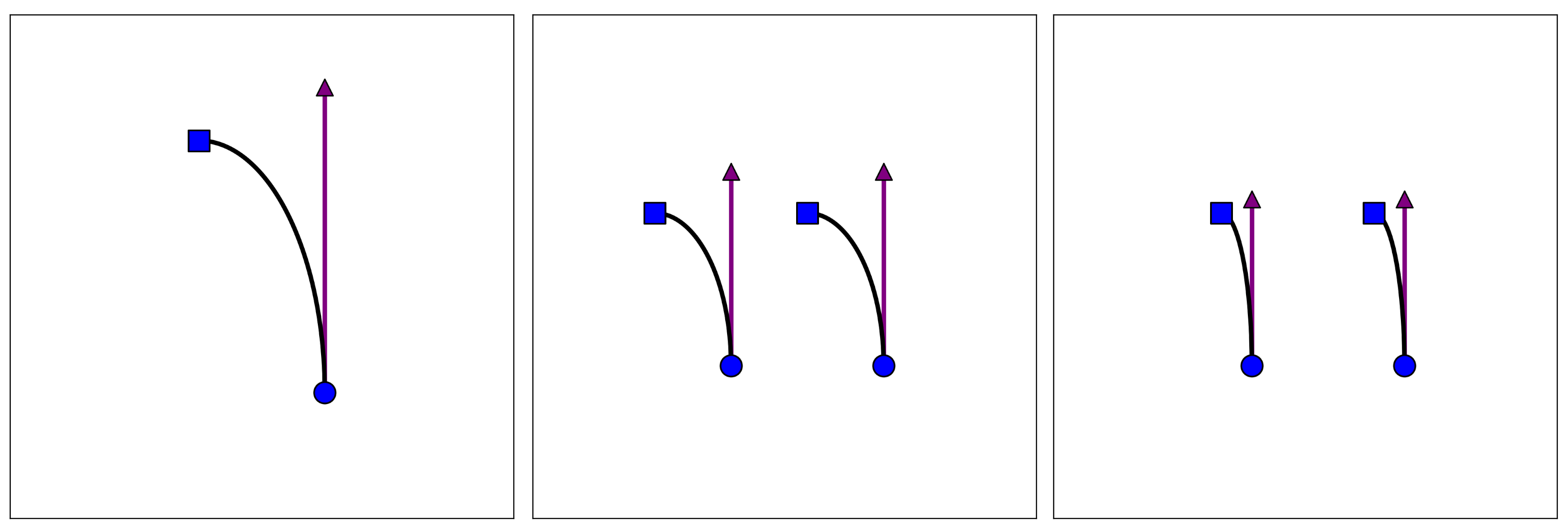
On the other hand, the linear regime requires the right scenario, where the nonlinearity becomes more linear. Both are plausible, and the result may even depend on the specific network and problem.
In fact, certain parameterizations of infinite width networks have been shown to be nonlinear, e.g., mean field parameterization. These limits describe feature learning, but come with their own drawbacks.
Note that linearization can also be achieved without infinite width, if networks are rescaled in weird ways. See these lecture notes (section 8.4) for more details.
Defining The Neural Tangent Kernel
Having motivated the study of neural tangent kernels (NTK), we define it.
Consider a model with parameters $\theta$, training on $m$ data points $(x_d, y_d)$ with MSEloss
\[L(\theta) = \frac12 \sum_{d=1}^m |f(x_d;\theta) - y_d|^2\]We update parameters via gradient flow (a continuous version of discrete gradient descent)
\[\dot{\theta}(t) = - \nabla_\theta L = \sum_{d=1}^m \nabla_\theta f(x_d;\theta(t))^\top \big(f(x_d;\theta(t)) - y_d\big)\]The NTK’s key insight is that model predictions on an input $x$ (for models under gradient flow) can be described by
\[\begin{align} \frac{d}{dt} f(x;\theta(t)) &= -\nabla_\theta f(x;\theta(t))\,\dot{\theta}(t) \\&= -\sum_{d=1}^m \underbrace{\big[\nabla_\theta f(x;\theta(t))\,\nabla_\theta f(x_d;\theta(t))^\top\big]}_{\text{NTK }\Theta_t(x,x_d)}\,\big(f(x_d;\theta(t)) - y_d\big). \end{align}\]$\Theta_t(x,x_d)\in\mathbb{R}^{k\times k}$ is a scalar called the Neural Tangent Kernel (NTK).
The evolution of model outputs on inputs $x$ are described by the time-dependent ODE
\[\frac{df(x)}{dt} = \sum_{x_d=\text{train data}} \Theta_t(x, x_d)\times \big(f(x_d) - y_d\big)\]The NTK is calculated by finding the model derivative w.r.t all trainable parameters. Then we sum over all the derivatives, and all output dimensions (due to the transpose) to get the kernel
\[\Theta_t(x,x') = \sum_{\text{params }j}\sum_{o=1}^O \frac{\partial f_o(x)}{\partial \theta_j}\frac{\partial f_o(x')}{\partial \theta_j}.\]where $o$ refers to the output dimension index.
When $\theta(t) = \theta(t=0) + t\,\dot{\theta}(0)$, the NTK becomes constant over time.
To make this kernel more concrete, we do explicit computations for 1D input and output models with 1 hidden layer.
Explicit Kernel - Quadratic Model
Consider a 1D input-output model with 1 hidden layer
\[f(x,\mathbf{w}_1,\mathbf{w}_2,\mathbf{b}_1,b_2) = C\sum_{i}^{N}\big(w_{2,i}\,\sigma(w_{1,i}x + b_i) + b_2\big)\]with a constant scaling factor $C$. The second layer sums over the $N$ neurons directly for the output (note that in general, we could imagine another activation applied on the second layer as well).
The derivatives of our model w.r.t. all parameters can be summarized by its derivatives w.r.t. the parameters of a single neuron. Let the contribution of a single neuron be denoted
\[h_i = w_{2,i}\,\sigma(w_{1,i}x+b_i)\]then the derivatives are
\[\nabla_\theta h_i(x;\theta(t)) = \begin{pmatrix} \frac{d h_i}{dw_{1,i}}\\ \frac{d h_i}{db_i}\\ \frac{d h_i}{dw_{2,i}} \end{pmatrix} = \begin{pmatrix} w_{2,i}x\,\sigma'(w_{1,i}x+b_i)\\ w_{2,i}\,\sigma'(w_{1,i}x+b_i)\\ \sigma(w_{1,i}x+b_i) \end{pmatrix}\]and the kernel is given by summing over the neurons and the neuron-independent $b_2$.
\[\begin{align} \Theta(x,x') = C^2&\sum_{i}^{N}\nabla_\theta h_i(x;\theta(t))\,\nabla_\theta h_i(x';\theta(t)) + \frac{\partial f}{\partial b_2}\\ \\= C^2&\bigg[\sum_{i}^{N}\sigma(w_{1,i}x+b_i)\,\sigma(w_{1,i}x'+b_i) \\+& (1+xx')\sum_{i}^{N}w_{2,i}^2\,\sigma'(w_{1,i}x+b_i)\,\sigma'(w_{1,i}x'+b_i)\bigg] + \frac{\partial f}{\partial b_2}. \end{align}\]The neuron derivatives can be interpreted as the “features” of our kernel (e.g., if $x’$ and $x$ have large values for these features, then they are considered “close”). These features are generally nonlinear in $x$.
NTK Parameterization
For the neural tangent parameterization, we choose $C = 1/\sqrt{N}$ and initialize our parameters from distributions of 0 mean, constant variance (independent of neuron count $N$):
\[f(x,\mathbf{w}_1,\mathbf{w}_2,\mathbf{b}_1,b_2) = \frac{1}{\sqrt{N}}\sum_{i}^{N}\big(w_{2,i}\,\sigma(w_{1,i}x + b_i) + b_2\big).\]Using a quadratic activation yields the following kernel
\[\begin{align} \Theta(x,x') = &\frac{1}{N}\bigg[ \sum_{i}^{N}(w_{1,i}x+b_i)^2(w_{1,i}x'+b_i)^2 \\&+ 4(1+xx')\sum_{i}^{N} w_{2,i}^2 (w_{1,i}x+b_i)(w_{1,i}x'+b_i) + 1 \bigg]. \end{align}\]Testing Our Expression
We would like to verify that:
- Our expression accurately predicts the functional evolution of a model.
- The kernel becomes constant as the hidden dimension $N\to\infty$.
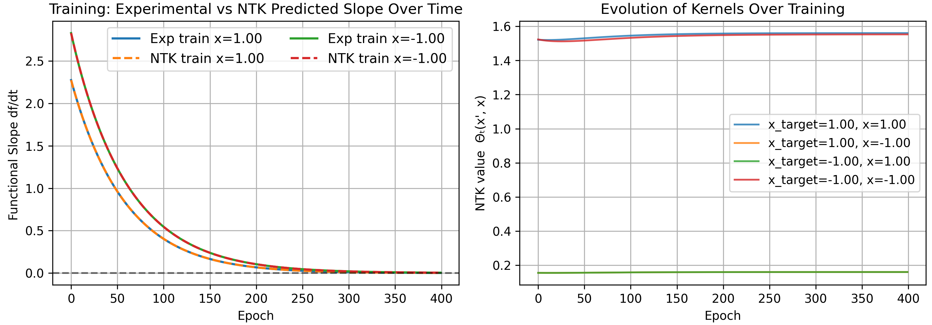
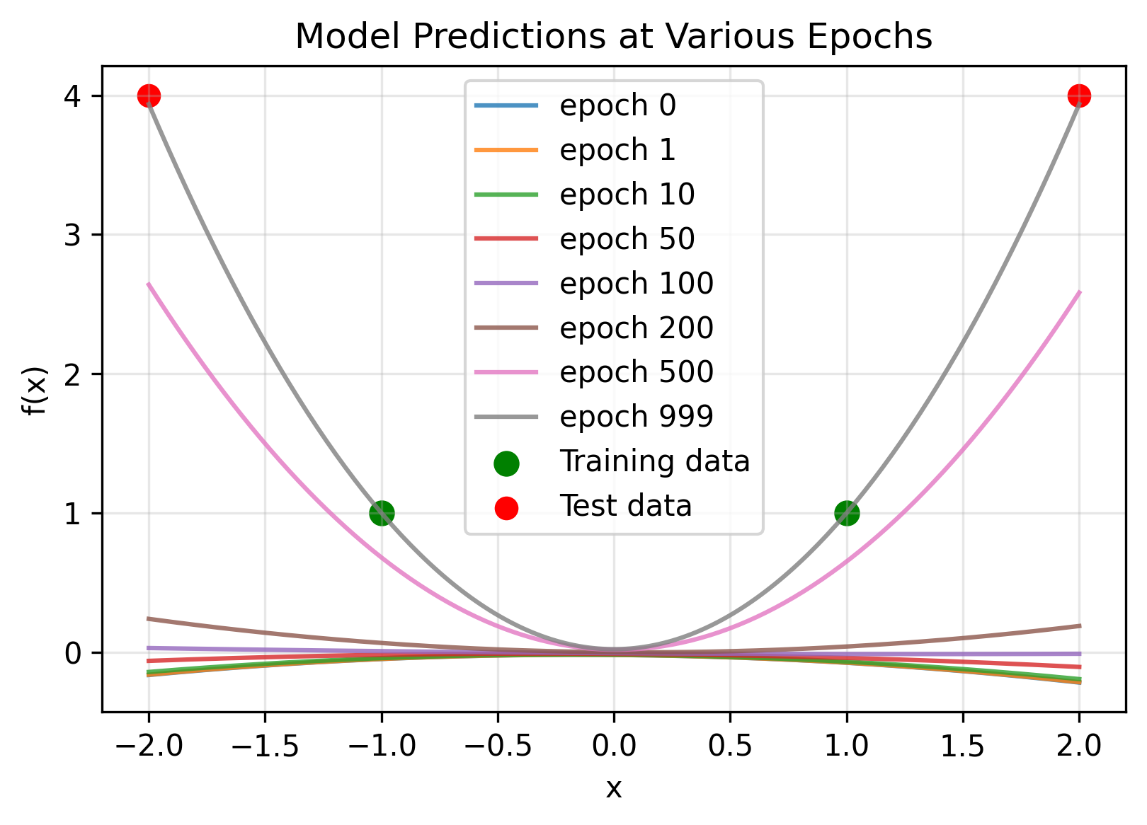
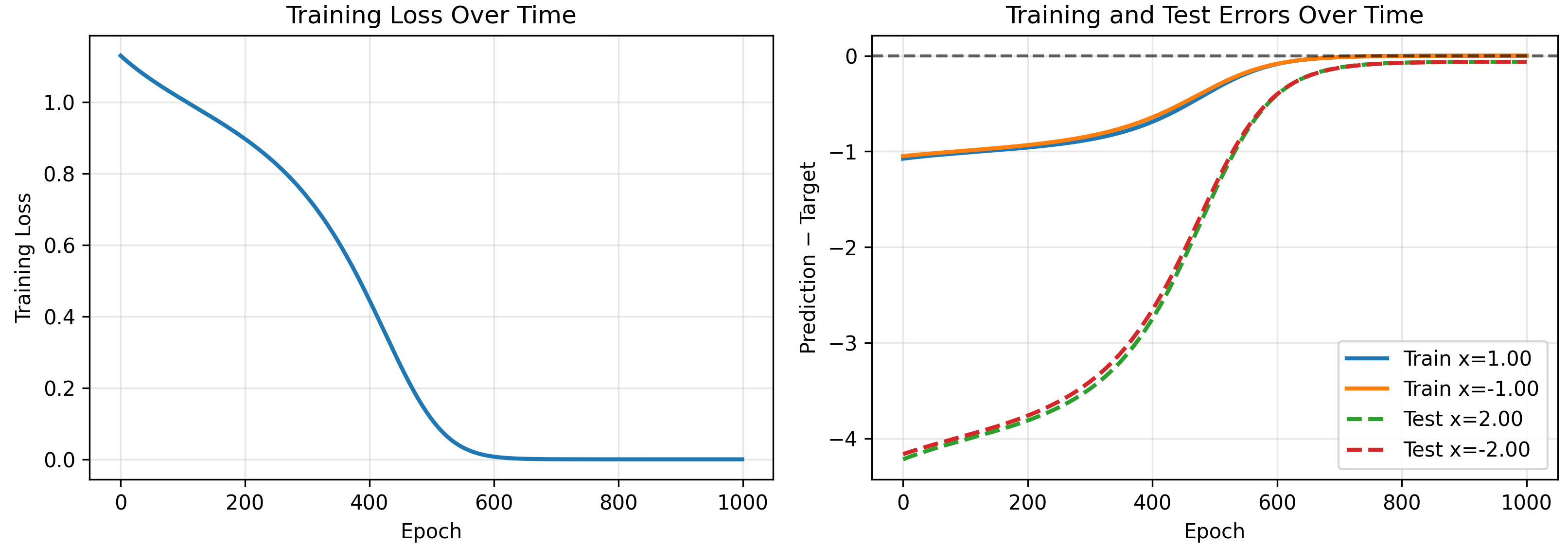
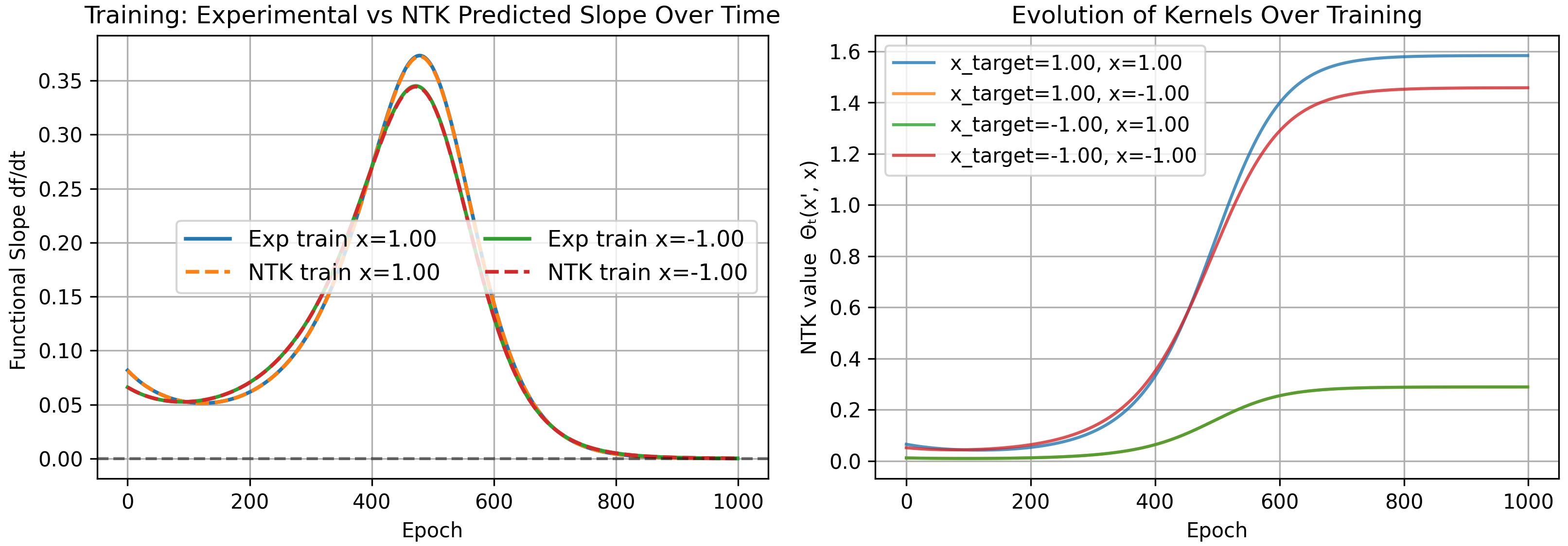
We test on a toy model, removing the second layer bias. Note the 1D-1D quadratic network can only output a quadratic polynomial (the sum of the neurons which are quadratics with weights $w_{2,i}$, must also be a quadratic). We initialize a model and see if our kernel accurately predicts its evolution on training and test inputs.
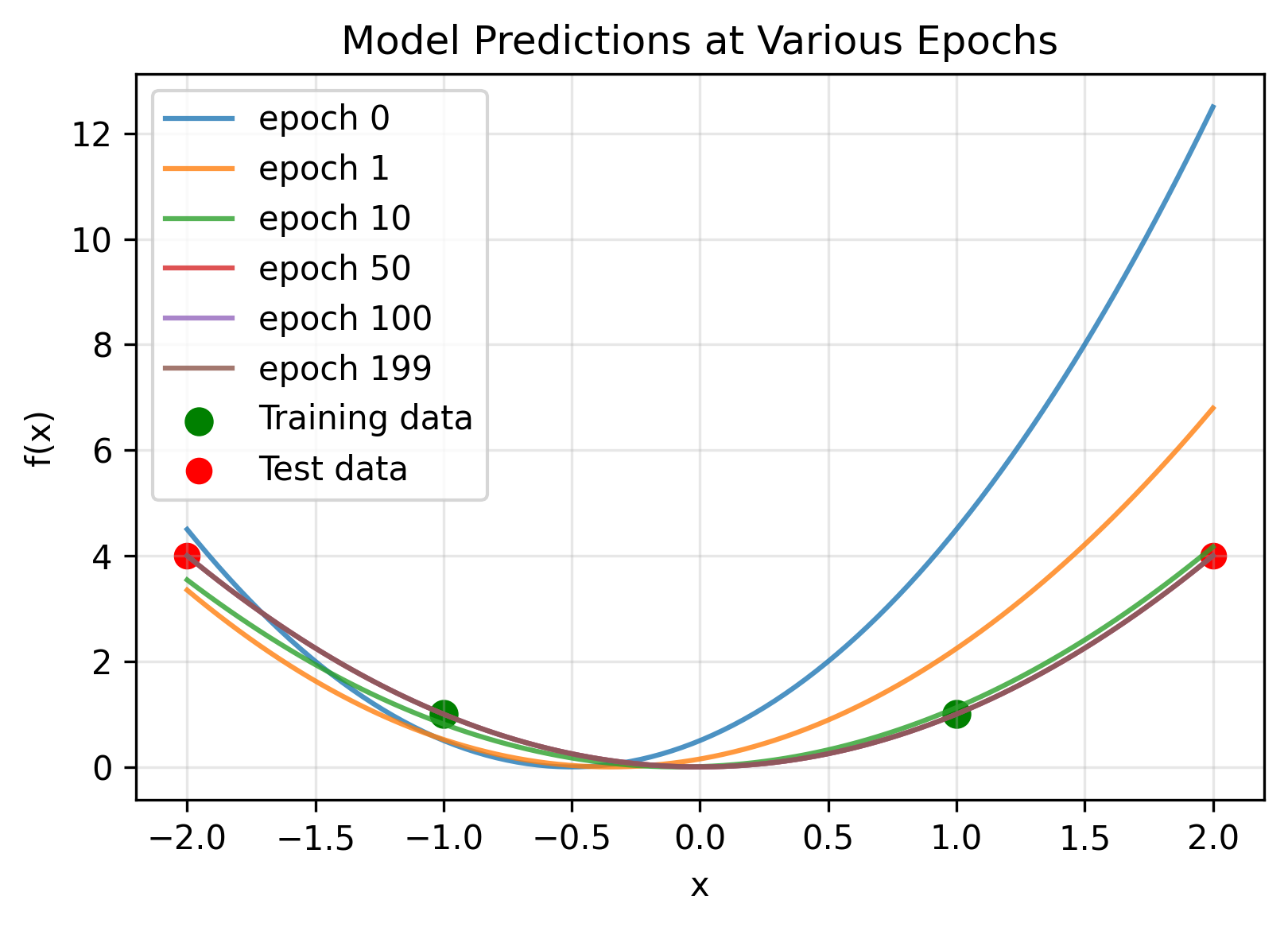
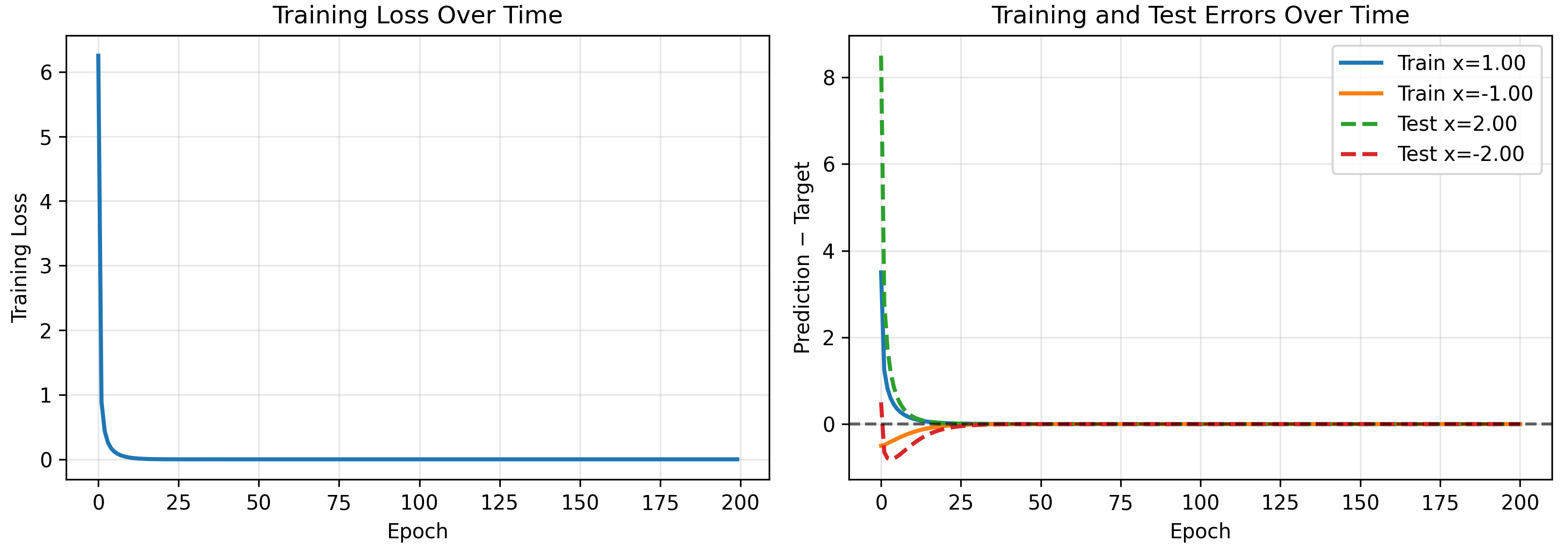
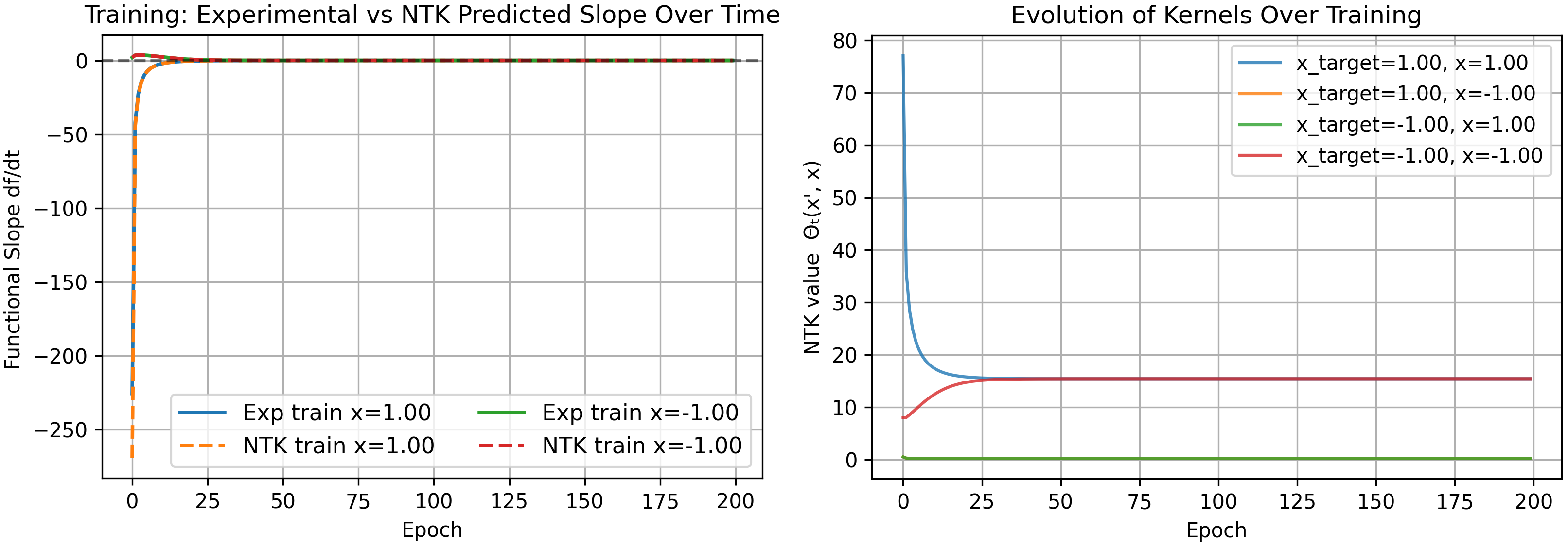
As a check that our kernel is correct, we can explicitly calculate it at $t=0$. For one neuron without layer 2 biases we have
\[\Theta(x,x') = (w_1x+b)^2(w_1x'+b)^2 + 4(1+xx')w_2^2(w_1x+b)(w_1x'+b)\]which for our starting parameters $w_1=1.0$, $b=0.5$, $w_2=2.0$, is
\[\Theta(x,x') = (x+0.5)^2(x'+0.5)^2 + 16(1+xx')(x+0.5)(x'+0.5)\]yielding the following kernels
\[\begin{pmatrix} \Theta(1,1)\\ \Theta(-1,1)\\ \Theta(1,-1)\\ \Theta(-1,-1) \end{pmatrix} = \begin{pmatrix} 77.0625\\ 0.5625\\ 0.5625\\ 8.0625 \end{pmatrix}\]matching our numerical results shown above.
More Neurons
We move to models with larger widths. We choose parameters
\[w_1 \sim \mathrm{Unif}(-1,1), \qquad b \sim \mathrm{Unif}(-0.5,0.5), \qquad w_2 \sim \mathrm{Unif}(-1,1),\]where layer 1 biases are sampled from a smaller distribution (to prevent them from drowning out the weights) purely for nicer graphs, and again no layer 2 biases.
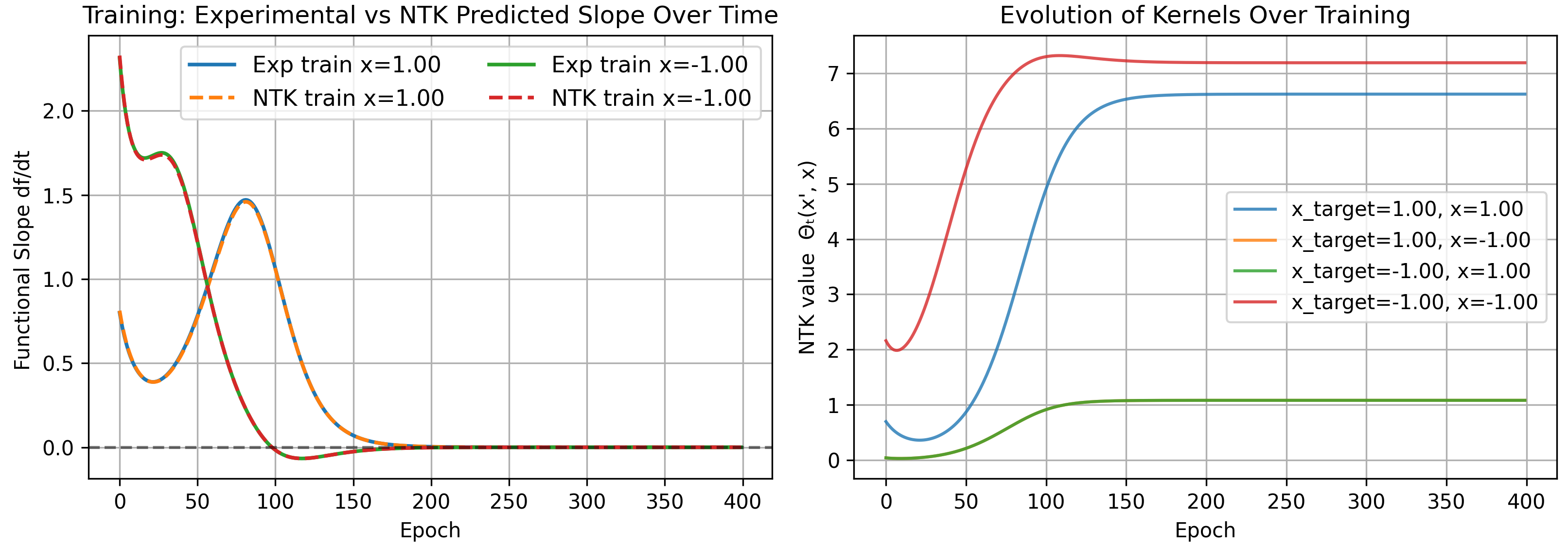
Note that the number of epochs increased, and the overall kernel values are much smaller than before. This is expected, since the rate at which our model fits the data is determined by the magnitude of kernels, and if all kernels are small, training is naturally slower.
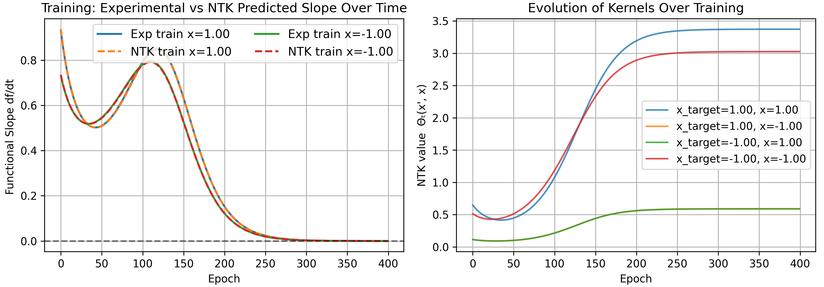
As a bonus, note the infinite width kernel simplifies into several expectation values
\[\begin{align} \Theta(x,x') \rightarrow& \langle w_1^4\rangle x^2 x'^2 + \langle w_1^2\rangle\langle b^2\rangle(x^2 + 4xx' + x'^2) \\& + \langle b^4\rangle + 4(1+xx')\langle w_2^2\rangle\big(\langle w_1^2\rangle xx' + \langle b^2\rangle\big) \end{align}\]where independence of various initialization distributions for parameters results in a simple expression. Using the moments of our initialization distribution, we can compute the infinite width kernel. For our distribution, where
\[w_1 \sim \mathrm{Unif}(-1,1), \qquad b = 0, \qquad w_2 \sim \mathrm{Unif}(-1,1),\]we get the following moments
\[\langle w_1^2\rangle = \frac{1}{3}, \qquad \langle w_1^4\rangle = \frac{1}{5}, \qquad \langle b^2\rangle = \frac{1}{12}, \qquad \langle b^4\rangle = \frac{1}{80}, \qquad \langle w_2^2\rangle = \frac{1}{3}\]resulting in the following values for our kernel
\[\Theta(1,1)=1.490278,\quad \Theta(1,-1)=0.156944,\quad \Theta(-1,-1)=1.490278\]matching our results above for 1000 neurons.
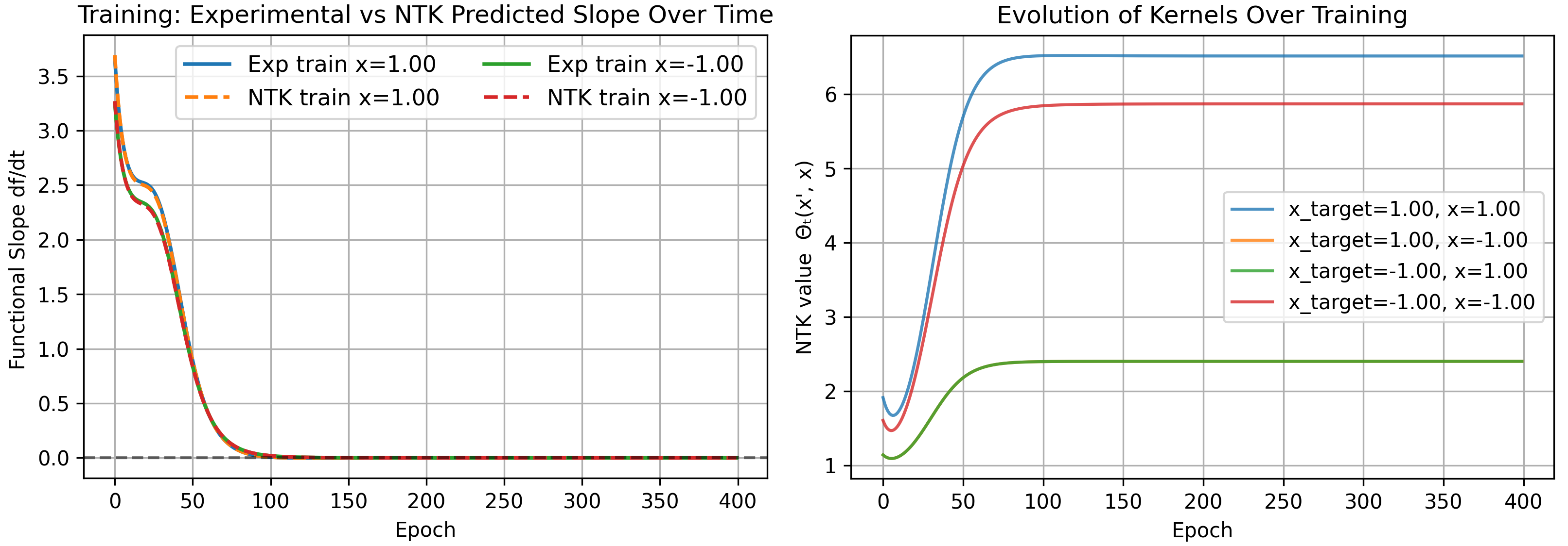
Standard Parameterization
Thus far we used the “NTK” parameterization. We initialized parameters from mean 0 fixed-variance distributions, and larger networks are rescaled by a constant $1/\sqrt{N}$ scaling factor.
$1/\sqrt{N}$ scaling does not occur in actual networks. Instead, network weights are initialized from a distribution with variance that decreases proportional to scale (e.g., $\propto 1/\sqrt{N}$). The NTK parameterization factorizes the scaling into an overall constant. This is important since this reparameterization guarantees that weights of $O(1)$ only experience gradient updates of $O(1/\sqrt{N})$, and thus do not change much over training. This leads us into the NTK limit.
In the standard parameterization, weights are $O(1/\sqrt{N})$ and experience updates of $O(1)$. Thus the weights do change significantly, and feature learning can occur. For the standard parameterization, the kernel is similar but with $C=1$:
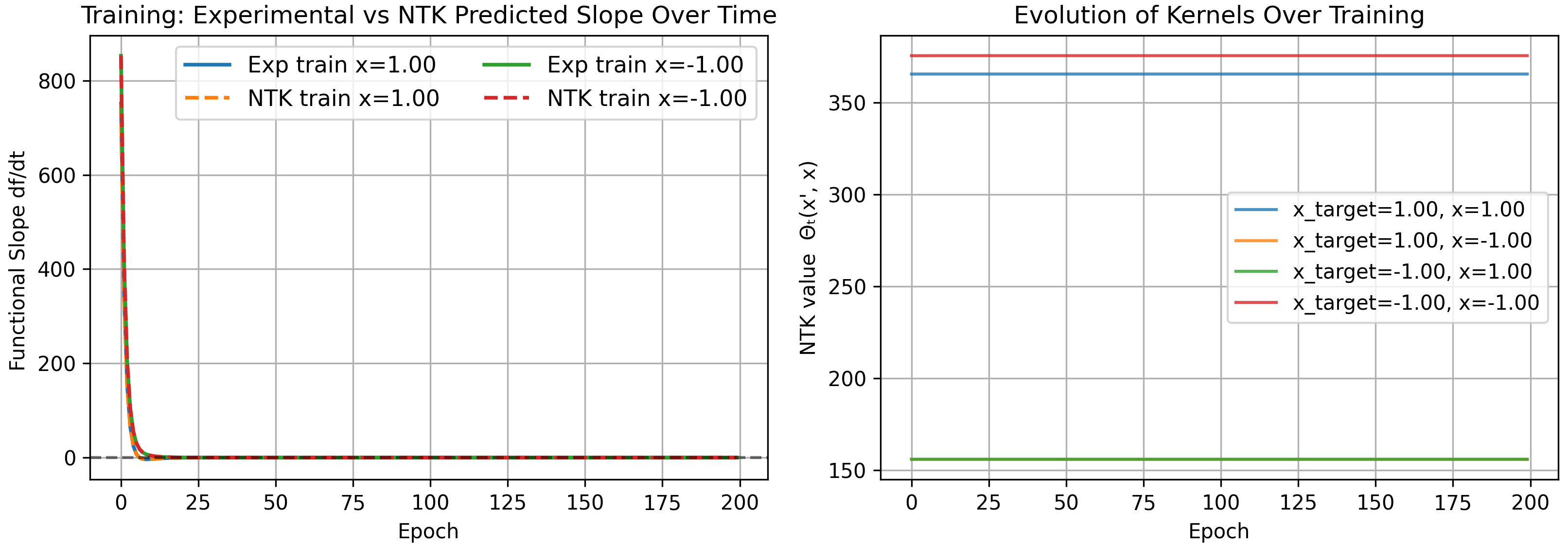
\[\begin{align} \Theta(x,x') = &\bigg[ \sum_{i}^{N}(w_{1,i}x+b_i)^2(w_{1,i}x'+b_i)^2 \\&+ 4(1+xx')\sum_{i}^{N} w_{2,i}^2 (w_{1,i}x+b_i)(w_{1,i}x'+b_i) + 1 \bigg]. \end{align}\]Note our first summation has $N$ terms of $O(1)$ (first layer weights and biases are scaled proportional to the input dimension, not the hidden dimension), and in the limit $N\to\infty$ becomes infinite. This was not a problem with NTK parameterization due to our scaling.
One way to understand this is to recall the first term consists of derivatives w.r.t. layer 2 weights, of which there are $N$. Compared to before where they were $O(1)$, this derivative is now with respect to incredibly small $O(1/\sqrt{N})$ values. These derivatives are large unlike before.
As a result, the kernel becomes infinite for very wide networks and the constant assumption is no longer meaningful. We run our previous problem with standard parameterization as an example.
Mean-Field Parameterization
Another parameterization often discussed in the literature is known as the mean-field parameterization. Here parameters are initialized from fixed-variance distributions but rescaled by $1/N$ instead of $1/\sqrt{N}$:
\[f(x,\mathbf{w}_1,\mathbf{w}_2)=\frac{1}{N}\sum_{i}^{N} w_{2,i}\,\sigma(w_{1,i}x).\]This results in a kernel which vanishes in infinite width
\[\begin{align} \Theta(x,x') = &\frac{1}{N^2}\bigg[ \sum_{i}^{N}(w_{1,i}x+b_i)^2(w_{1,i}x'+b_i)^2 \\&+ 4(1+xx')\sum_{i}^{N} w_{2,i}^2 (w_{1,i}x+b_i)(w_{1,i}x'+b_i) + 1 \bigg] \\&\rightarrow 0. \end{align}\]This has direct consequences—the time it takes to train a mean-field network takes longer than a NTK network, scaling with width. In the worst case, it requires infinite time to train an infinitely wide network. This makes sense to some degree: all parameters must move further to change the function under this harsher scaling.
Despite these drawbacks, there are very good reasons to study the mean-field parameterization. Mean field is able to describe feature learning.
It also has a simple interpretation—returning to our early picture of visualizing neurons as points in weight space that move according to gradient flow, infinite width lets us model a neural network as a continuous weight distribution. The dynamics of this distribution can be described via tools from fluid mechanics (e.g., a nonlinear PDE). More on this hopefully in a future blog post.
End
That marks the end of this blog post. It was a nice structured way to make sure I really understood how NTK works and how to do calculations with it—lacking in novelty, but I’ll save that for future posts.