Optimal Flow-Matching

The implementation of the solution for various datasets are available on github.

Introduction

The training objectives of diffusion models can be solved analytically for an arbitrary dataset, yielding an algorithm that optimally denoises images in a way that minimizes the loss without any training. However, the analytical solution has two undesirable properties:

Removing the noise at a single step requires iterating through the entire dataset. This is computationally expensive.
The algorithm only generates images present in the training set. It memorizes and cannot produce new images.

However, this algorithm may be useful for understanding how deep learning models trained with the diffusion objective are producing new images.

Flow-matching is a new formulation of generative modeling using the language of ODE flows. It is equivalent to diffusion, but conceptually and mathematically simpler. Here, we derive the solution that minimizes the flow-matching objective’s loss for an arbitrary dataset.

A common toy example in flow-matching is to match a 2D isotropic Gaussian (blue) to a checkerboard distribution (red).

Flow-Matching

In flow-matching, we randomly sample points $\vec{x_{i}}, \vec{x_{f}}$ from the input and output distributions, and calculate a sample velocity

\[\vec{v}_{s} = \vec{x_i} \alpha' (t) + \vec{x_f} \beta' (t)\]

where $t$ is a randomly chosen time $t \varepsilon [0, 1]$, and $\alpha (t), \beta (t)$ are scheduling functions with $\alpha (0) = \beta (1) = 1, \alpha (1) = \beta (0) = 0$. Common choices are $\alpha(t) = 1 - t, \beta(t) = t$.

We train a model $\vec{v}_{m}(\vec{x}, t)$ to predict the sample velocity given the position

\[\vec{x} = \vec{x}_i \alpha(t) + \vec{x}_f \beta(t)\]

Our model minimizes the MSE loss

\[L = E_{\vec{x_{i}}, \vec{x_{f}}, t} \left[ \vec{v}_{m} (\vec{x}, t) - \vec{v}_{s})^2 \right]\]

where the expected value is taken over the distribution of inputs and outputs $\vec{x_{i}}, \vec{x_{f}}$.

The MSE loss is minimized if our model predicts the average sample velocity for a given $\vec{x}, t$

\[\implies \vec{v}_{m} (\vec{x}, t) = \langle \vec{v_{s}} \rangle_{\vec{x}, t}\]

which can be calculated by integrating over the distribution of inputs and outputs $P(\vec{x_i}, \vec{x_f})$ conditioned on points $\vec{x_i}, \vec{x_f}$ contributing to the velocity at point $\vec{x}, t$. The average velocity calculation involves integrals of the following form

\[\langle x_{i} \rangle_{\vec{x}, t} = \frac{\int_{\vec{x_i}, \vec{x_f}} \vec{x}_{i} \, P( \vec{x_i}, \vec{x_f} \mid \vec{x} = \vec{x_i} \alpha (t) + \vec{x_f} \beta (t)) \, dx_i dx_f}{\int_{\vec{x_i}, \vec{x_f}} \, P( \vec{x_i}, \vec{x_f} \mid \vec{x} = \vec{x_i} \alpha (t) + \vec{x_f} \beta (t)) \, dx_i dx_f}\]

where we condition the distribution of inputs and outputs on points contributing to the velocity $\langle \vec{v_{s}} \rangle_{\vec{x}, t}$. The denominator ensures the conditional probability distribution is appropriately normalized (since only connected pairs $\vec{x}_i, \vec{x}_f$ contribute to a given $\vec{x}, t$).

These integrals can be simplified if we impose constraints on the distributions (eg, our inputs are Gaussian noise).

Optimal Solution

If the input distribution is a Gaussian, and the output distribution is defined by discrete training data points $\vec{\mu}_j$, the velocity that minimizes our training objective is given by

\[\vec{v} (\vec{x}, t) = \frac{1}{1 - t}\left( \sum_j \vec{\mu}_{j} \cdot \text{Softmax}_{\vec{\mu}_j}\left(-\frac{1}{2} \frac{\left(\vec{x} - \vec{\mu}_{j} t \right)^2}{(1 - t)^2 \sigma_i} \right) - \vec{x} \right)\]

where we have additionally assumed the schedule is linear. $\text{Softmax}_{\vec{x}} \left(f(\vec{x}) \right)$ is the softmax probability distribution formed from the vectors $\vec{x}$, given by

\[\text{Softmax}_{\vec{x}}\left(f(\vec{x}) \right) = \frac{e^{f(\vec{x})}}{\sum_{\vec{x}} e^{f(\vec{x})}}\]

For the derivation, see this appendix.

This algorithm is easy to interpret. At any time, the ideal flow checks the $L_2$ distance between the current point and all training data points, multiplied by a time dependent factor. The softmax turns this into a distribution, and it moves directly to the expected endpoint $\langle \mu \rangle$ of this distribution. The $1/(1 - t)$ term means that single-step integration from this point takes it directly to this expected end point.

The two drawbacks of ideal diffusion denoisers are present here:

Evaluating the velocity involves computing distances with all data points, which is computationally expensive for large datasets.
It memorizes the training data. As $t \rightarrow 1$, the velocity points directly to the closest data point (as the softmax penalizes more distant points). As a result, it only generates points at $t = 1$ that exist in the training data.

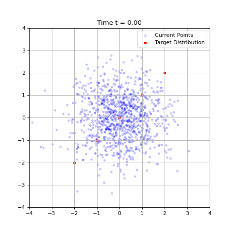
Despite this, such an algorithm may be helpful in interpreting how denoising generative models behave. For example, at $t = 0$, all our data points become identical and flows always move to the mean of the training data, which can be easily confirmed. As $t \rightarrow 1$, our flows begin to distinguish different data points and more fine features become pronounced.

Examples With Code

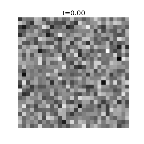
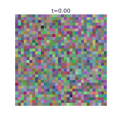
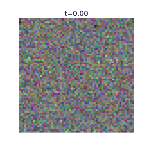
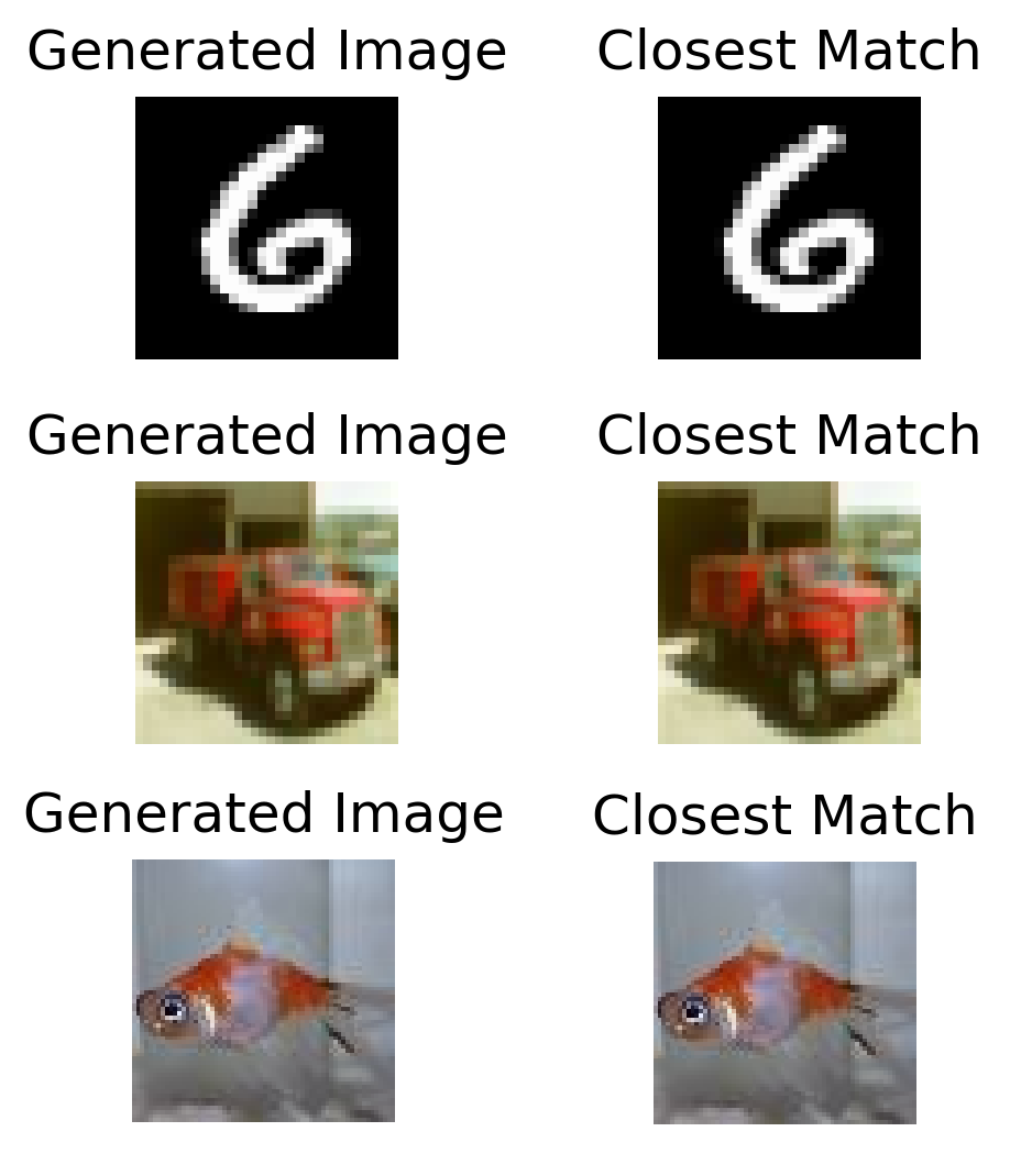
This algorithm has been implemented in this github repo with example uses. Here we display optimal flows using as training data the first 50,000 images of MNIST, CIFAR-10, and 5000 images from ImageNet.

Examples of the analytic denoiser on Gaussian noise for MNIST, CIFAR-10, and Imagenet.

With this algorithm, one can denoise images very quickly for small datasets, but the resulting images are nearly identical to training examples. It’s incapable of generating new images.

Although the ideal denoiser requires no training, all outputs are identical to images in the training data.

Since the ideal flow minimizes the MSE loss, one can compute the minimal training loss. This seems most enlightening when plotted as a function of $t$, where one observes that the loss is maximal near $t = 0$ and steadily decreases.

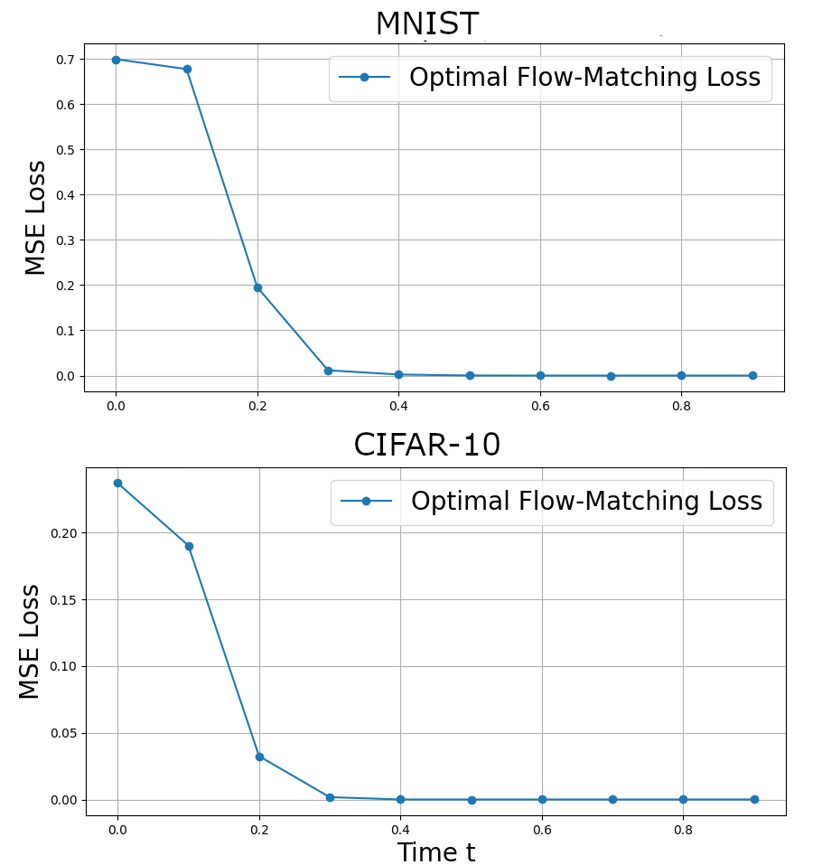
Optimal MSE loss at various parameters of $t$ for training MNIST and CIFAR-10. The loss at high values of $t$ is small since contributions to the velocity come mostly from a single sample, which the optimal denoiser has memorized. Losses were calculated using $400$ randomly generated points at each value of $t$.

This occurs because there is greatest variance in the velocity at the start, where all output images seem possible. As time progresses, very few images are likely and the softmax becomes dominated by a specific training example.

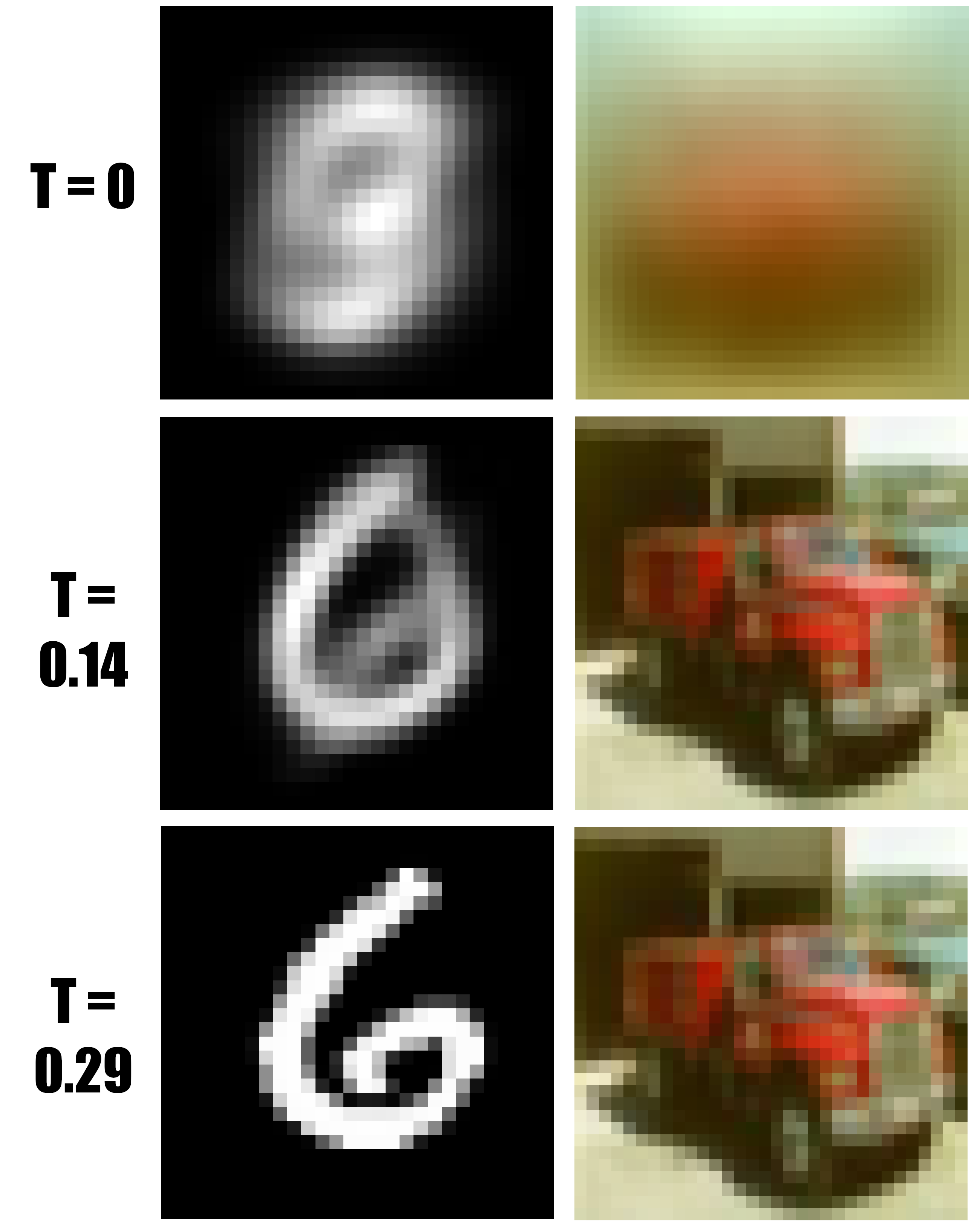
This can be seen explicitly when plotting our algorithms prediction for the final image at a given time, where they initially predict a blurry image corresponding to the average but very quickly decide on the final image. More training data should ensure the variance stays large for larger $t$ values.

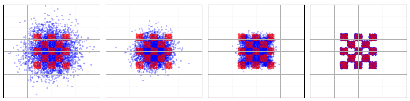
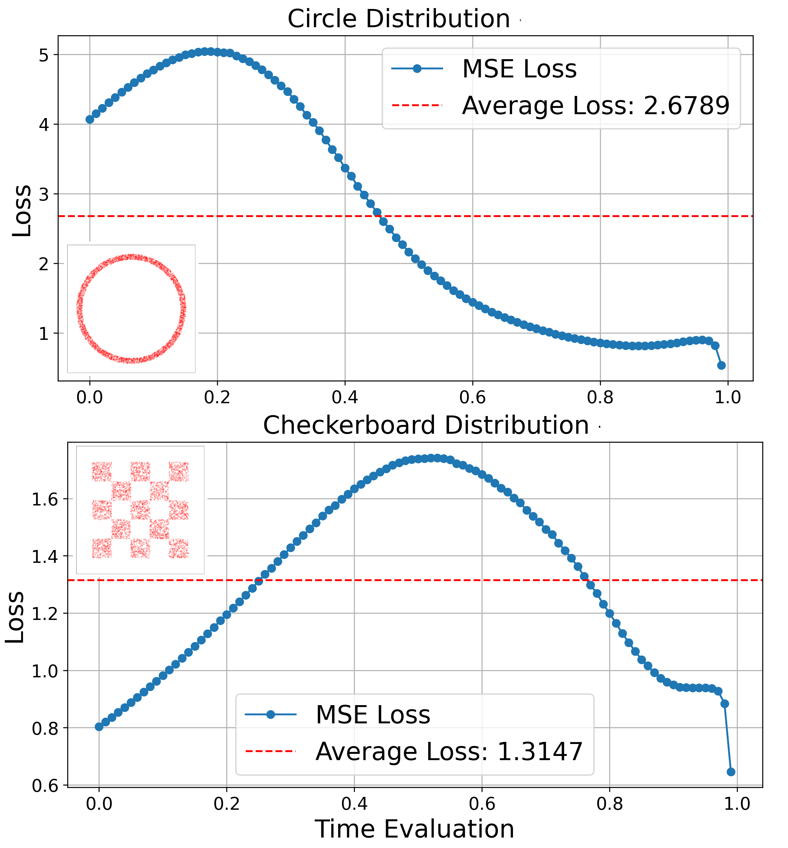
Optimal denoiser predictions for the final image for MNIST and CIFAR-10. Note that the optimal algorithm initially predicts the average of the training data, but quickly decides on which of the memorized samples corresponds to the input.

This behavior is very different for toy 2D distributions often used to visualize flow-matching algorithms such as circles, checkerboards or spiral distributions, where the loss is non-monotonic.

Optimal MSE loss at various parameters of $t$ for training common 2D toy distributions (matching a Gaussian to a circle or a checkerboard). Unlike the high dimensional problems earlier, the loss behaves non-monotonically. Losses were calculated using $40,000$ randomly generated points at each value of $t$.

What Do Models Actually Do?

For networks trained on large amounts of data, it is unlikely they have the capacity in their weights to store all their training data. Although this algorithm minimizes the loss, it cannot describe the behavior of networks except in the memorization regime that occurs with a small number of samples.

There exists a large body of work trying to understand how these models behave outside of the memorization regime, such as the appearance of geometric harmonic bases , and translational invariance and locality inherited from convolutional neural networks.

Here we focus on small insights from the optimal solution. For neural networks, the problem is estimating

\[\sum_j \vec{\mu}_{j} \cdot \text{Softmax}_{\vec{\mu}_j}\left(-\frac{1}{2} \frac{\left(\vec{x} - \vec{\mu}_{j} t \right)^2}{(1 - t)^2 \sigma_i} \right)\]

given a finite capacity.

Near $t = 0$, this term is easy to approximate since all data points $\vec{\mu}_{j} t \rightarrow 0$ and the flow points to the average. Only small corrections to the average-tending flow are needed and the error will be small as long as $t$ is small.

On the other hand, $t = 1$ appears difficult to approximate since all data points have separated and the softmax is dominated by the closest point, for which there are many candidates. The resolution to this paradox is that $\vec{x}$ near $t = 1$ is not random noise, but very close to the training data $\vec{\mu}_j$. Therefore our model can use cues present in $\vec{x}$ at this step to make a good guess towards the expected value of the softmax, or direction of flow.

What these cues are and how the model learns them do not seem explainable from the algorithm, but rather dependent on features of the data and model architecture.

Generalizations

For an arbitrary schedule where some data points are more likely than others, we have

\[\vec{v} (\vec{x}, t) = \frac{\alpha'}{\alpha} \vec{x} + \frac{\alpha \beta' + \alpha' \beta}{\alpha} \sum_j \vec{\mu}_{j} \cdot \text{Softmax}_{\vec{\mu}_j}\left(-\frac{1}{2} \frac{\left(\vec{x} - \vec{\mu}_{j} \beta \right)^2}{\alpha^2 \sigma_i} + \log C_j \right)\]

where $\alpha’, \beta’$ are derivatives of the scheduling functions, and $C_j$ is a constant that weighs the relative probability of certain data points in the training data.

If the output distribution consists of a superposition of isotropic Gaussians with variance $\sigma_f$, then

\[\begin{aligned} \vec{v}(\vec{x}, t) &= \left(\frac{1}{\alpha^2 \sigma_i + \beta^2 \sigma_f} \right) \cdot \bigg[ \vec{x} \left(\alpha' \alpha \sigma_i + \beta' \beta \sigma_f \right) \\ &\quad - \alpha \sigma_i\left(\alpha' \beta - \alpha \beta' \right) \left( \sum_j \vec{\mu}_{j} \cdot \text{Softmax}_{\vec{\mu}_j}\left(-\frac{1}{2} \frac{\left(\vec{x} - \vec{\mu}_{j} \beta \right)^2}{\alpha^2 \sigma_i + \beta^2 \sigma_f} + \log C_j \right) \right) \bigg] \\ \end{aligned}\]

which represents a case where Gaussian noise is added to our training data.

Optimal flow-matching from a 2D Gaussian to a series of points on a line with a nonlinear schedule $\alpha = 1 - t^{2}, \beta = t^{2}$ and allowing for variance in the output $\sigma_f > 0$.

The case of non-isotropic Gaussians can be found in the appendix, section 3.1.

Recent work has noted that far away from the data manifold the trajectories move in straight curl-free paths. I was curious if the optimal vector fields generated by flow-matching might always be conservative (and thus curl free) even close to the data manifold. If this was true, then the problem could be modeled via a time-dependent energy, which might simplify training.

Sadly the optimal flow is not always conservative. This can be calculated explicitly by looking at the curl in 2D for a set of discrete data points $>1$, in which one finds the curl increases at intermediate values of $t$ near the decision boundary that governs where points from Gaussian noise end up. Only when $t = 0, 1$ is the flow guaranteed to be nearly conservative, as the softmax simplifies.

Closing Thoughts

In my personal opinion, for well-defined problems that we know how to solve, we shouldn’t use learning algorithms like neural networks because they are slow, require lots of data and take a long time to train. A lot of problems in math, physics and computer science have these nice solutions. But there are a lot of ill-defined problems which we have no idea how to solve.

Flow-matching caught my attention since the formalism is very simple - it can be understood in the language of 2nd year physics and ODEs, and there is indeed an optimal analytic solution. Unfortunately this solution doesn’t have the useful properties that ones produced by deep learning do.

That said, I have ideas I’d like to try for making a more useful algorithm:

The analytical solution depends on softmax probabilities, which rapidly shrink to 0 for far-away points. Instead of a full pass through the data per computation, it seems feasible to go through the data, index it with an algorithm like locality sensitive hashing, and then approximately compute it by only using close points.
Recent work with locality suggests images can be generated by matching to patches of different scales - patches were used in image generation before deep learning arose (GANs), but the varying scales from diffusion seems like a new twist.

More on these approaches hopefully in future posts or papers.

On a side note, the optimal loss is very small at high $t$ values because the optimal flow instantly memorizes a specific point. This makes me wonder if it could serve as an indicator for the memorization regime, where a model that stops memorizing has significantly higher loss at high $t$ values. Would be nice to get a couple models in that regime and compare the loss vs t.

Acknowledgements

My interest in this topic was heavily influenced by this blog post, Flow With What You Know, by Scott Hawley. Many kind thanks to Scott Hawley and Sander Dieleman for their generosity in answering questions and sharing background knowledge on this topic.

If you find this post useful in your research or teaching, please consider citing it:

@misc{fan2025optimal,
  author = {Raymond Fan},
  title = {Optimal Flow-Matching},
  url = {https://rfangit.github.io/blog/2025/optimal_flow_matching/},
  year = {2025}
}