Introduction to Mean Flow
This tutorial is implemented as a google colab notebook, where you can follow along with the code and run it yourself.
Introduction
“Mean Flows for One-step Generative Modeling” is a new idea to modify flow matching for 1 step generation. In this tutorial post, we’ll introduce the basics and an example implementation for standard 2d toy flow matching problems. Do consider reading the original paper for more details.
Flow Matching
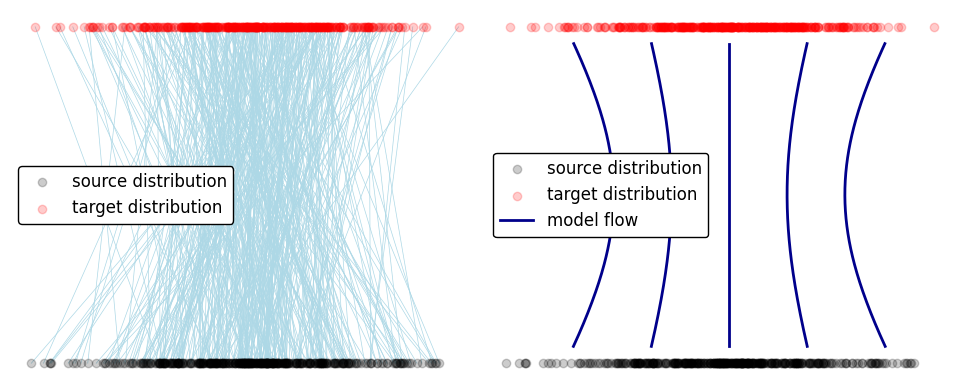
In flow matching, we train a model to learn a flow to transform a source distribution into a target distribution. This model is trained by sampling random points from both distributions along with random times. Our model will learn the average direction to flow for a given $\vec{x}(t), t$, where $\vec{x}(t)$ represents our current data at time t.
Unfortunately this flow is fairly curved. As a result, transforming source to target requires evaluating our model at many points.
Mean Flow
Note: We follow the convention in the original paper, where $t = 0$ corresponds to our data, and $t = 1$ corresponds to the noise.
Instead of training a model to predict the flow at a point $v(\vec{x}(t), t)$, mean flow modifies the training algorithm and model to predict the average flow over the interval $r, t$ given by
\begin{equation} u(\vec{x}(t), t, r) = \frac{1}{t - r} \int_{r}^{t} v(\vec{x}(s), s) ds \end{equation}
This corresponds to averaging the flow over the green line in the following diagram.
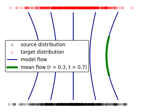
The mean flow is useful in generating with less steps, since the model already averages over $r, t$. 1-step sampling for example can be accomplished by setting $r = 0, t = 1$, and using the model’s mean flow to instantly generate outputs from inputs.
\begin{equation} \vec{x}(t = 0) = \vec{x}(t = 1) - u(\vec{x} (t = 0), r = 0, t = 1) \end{equation}
Note that mean flow models can still be used for multi-step generation.
To train a mean flow model, we modify the model to accept an extra time parameter $r$ (the starting time for our velocity averaging), and modify our loss function.
Modified Loss
Taking the derivative with respect to $t$ (treating r as a constant), we get
\[\begin{aligned} &\frac{d}{dt} \left( (t - r) u(\vec{x}(t), r, t) \right) = \frac{d}{dt} \int_r^t v(\vec{x}(s), s)\, ds \\& \implies u(\vec{x}(t), r, t) = v(\vec{x}(t), t) - (t - r) \frac{d}{dt} u(\vec{x}(t), r, t) \end{aligned}\]The time derivative can be computed in neural networks easily thanks to automatic differentiation.
Specifically, pytorch has a function called jvp (standing for jacobian vector product), which takes the product of the derivatives of a function with a vector. JVP can compute the derivative, with one issue: in $\frac{d}{dt} u(\vec{x}(t), r, t)$, our model depends on $t$ explicitly in its third argument, and implicitly in its first argument $\vec{x}(t)$.
JVP only computes explicit derivatives, so we need to make the $t$ dependence apparent. This yields
\begin{equation} \frac{d}{dt} u(\vec{x}(t), r, t) = v(\vec{x} (t), t) \times \frac{\partial}{\partial \vec{x}} u(\vec{x}(t), r, t) + \frac{\partial}{\partial t} u(\vec{x}(t), r, t) \end{equation}
which is the jacobian vector product of our model $u(\vec{x}(t), r, t)$ with the vector $v, 0, 1$.
Mean Flow Code
That covers the theory in mean flows. In practice, we make 3 modifications to standard flow matching. In flow matching:
- Random t values are generated in training.
- Loss is computed by comparing the model to the sample velocity
- Sampling occurs by evaluating the model at time t and incrementing forward by dt.
In mean flow:
- Random $t, r$ values are generated in training, with $t > r$.
- Loss is computed with the sample velocity modified by a jacobian term.
- Sampling occurs by evaluating the model at $t = t_{current}, r = t - dt $. For single step sampling, we evaluate at $r = 0, t = 1$.
To accomplish this, we define
- a model that accepts an additional time parameter $r$. For 2D examples, a couple fully connected layers suffice, and it’s easy to add the extra time dimension.
- a class for handling $t, r$ generation that computes the loss.
- a training function that uses our pre-existing class.
Note: Pay careful attention to loss computation! If you don’t use detach() to stop the flow of gradients, it’s very easy to get a model that never trains.
# Mean Flow Model

class MeanFlowNet(nn.Module):
def **init**(self, input_dim, h_dim=64):
super().**init**() # Input dimension should be x (input_dim) + t (1) + r (1) = input_dim + 2
self.fc_in = nn.Linear(input_dim + 2, h_dim)
self.fc2 = nn.Linear(h_dim, h_dim)
self.fc3 = nn.Linear(h_dim, h_dim)
self.fc4 = nn.Linear(h_dim, h_dim)
self.fc_out = nn.Linear(h_dim, input_dim)

    def forward(self, x, t, r, act=F.gelu):
        t = t.expand(x.size(0), 1)  # Ensure t has the correct dimensions for x batches
        r = r.expand(x.size(0), 1)  # Add r for meanflow!

        x = torch.cat([x, t, r], dim=1)
        x = act(self.fc_in(x))
        x = act(self.fc2(x))
        x = act(self.fc3(x))
        x = act(self.fc4(x))
        return self.fc_out(x)

# MeanFlow class that handles time generation, loss computation

class MeanFlow:
def **init**(self,):
super().**init**()

    def sample_t_r(self, batch_size, device):
        # Generate random t values in the shape of the batch size
        samples = torch.rand(batch_size, 2, device=device)

        # Assign the smaller values to r, larger values to t, unsqueeze to make it fit the 2D data
        t = torch.max(samples[:, 0], samples[:, 1]).unsqueeze(1)
        r = torch.min(samples[:, 0], samples[:, 1]).unsqueeze(1)
        return t, r

    def loss(self, model, target_samples, source_samples):
        batch_size = target_samples.shape[0]
        device = target_samples.device

        t, r = self.sample_t_r(batch_size, device) # Generate t, r

        interpolated_samples = (1 - t) * target_samples + t * source_samples
        velocity = source_samples - target_samples # velocity takes targets to sources

        ## Mean Flow Specific Loss Calculation ##
        jvp_args = (model,(interpolated_samples, t, r),(velocity, torch.ones_like(t), torch.zeros_like(r)), )
        u, dudt = jvp(*jvp_args, create_graph=True)
        u_tgt = velocity - (t - r) * dudt

        ## NOTE: Very important to use .detach().
        ## This sort of gradient based loss is very unstable otherwise
        ## and models can get stuck in extremely terrible local minima!!
        loss = F.mse_loss(u, u_tgt.detach()) ## Default MSE Loss
        return loss

# Training function that uses the class

def train_mean_model(model, source_data_function, target_data_function, n_epochs=100, lr=0.003, batch_size=2048, batches_per_epoch=10, epoch_save_freq = 10, checkpoint_prefix='mean_flow_model'):
optimizer = optim.Adam(model.parameters(), lr=lr)#torch.optim.AdamW(model.parameters(), lr=lr, weight_decay=0.0) #different optimizer
device = next(model.parameters()).device
#define an instance of meanflow to use to handle times and loss calculation

    meanflow = MeanFlow()

    for epoch in range(n_epochs):
        model.train()
        total_loss = 0.0
        for batch_idx in range(batches_per_epoch):
            # obtain points
            source_samples = source_data_function(batch_size).to(device)
            target_samples = target_data_function(batch_size).to(device)

            # Use points in the meanflow class
            loss = meanflow.loss(model, target_samples, source_samples)

            loss.backward()
            optimizer.step()
            optimizer.zero_grad()

            total_loss += loss.item()
        avg_loss = total_loss / batches_per_epoch
        print(f"Epoch [{epoch}/{n_epochs}], Avg Loss: {avg_loss:.4f}")

        if epoch % epoch_save_freq == 0:
            # Save model checkpoint
            checkpoint_path = f'{checkpoint_prefix}_epoch_{epoch}.pt'
            torch.save({
                'epoch': epoch,
                'model_state_dict': model.state_dict(),
                'optimizer_state_dict': optimizer.state_dict(),
                'loss': loss.item(),
            }, checkpoint_path)
            print(f"Saved model checkpoint to {checkpoint_path}")
    # Always save final model at the end
    checkpoint_path = f'{checkpoint_prefix}_epoch_{n_epochs}.pt'
    torch.save({
        'epoch': n_epochs,
        'model_state_dict': model.state_dict(),
        'optimizer_state_dict': optimizer.state_dict(),
        'loss': loss.item(),
    }, checkpoint_path)
    print(f"Saved model checkpoint to {checkpoint_path}")
    return model
And that’s it!
2D Example
We’ll demonstrate mean flow on several 2D distributions.
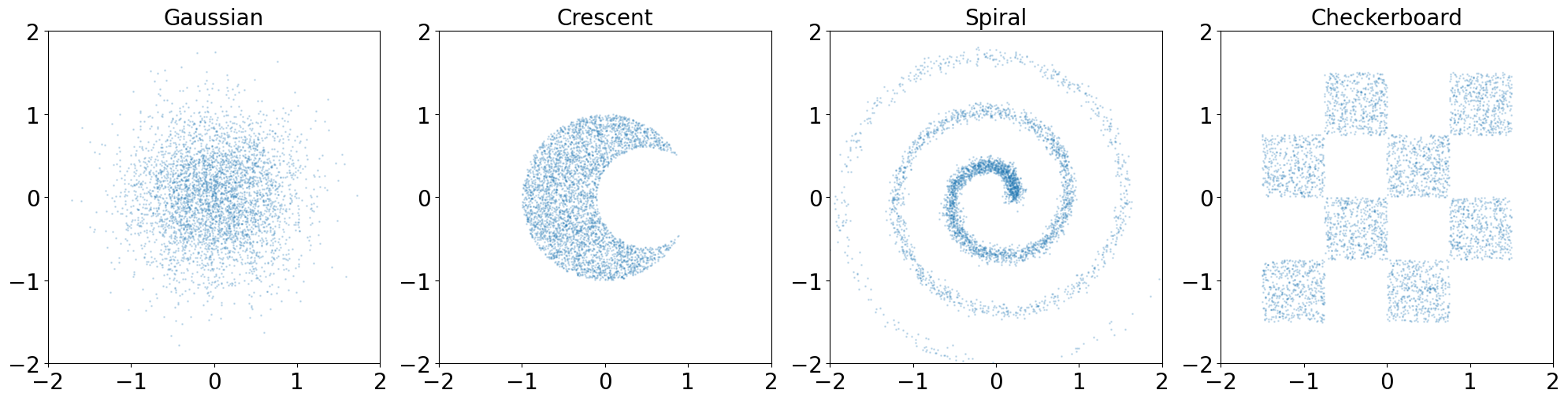
We’ll start with the checkerboard distribution.
Flow Matching Example
As a comparison, we first train a flow matching model. We define a model and a flow matching training function that does not use our earlier class. After training, we display 1 step integration as well as multi-step integration, using a simple forward euler to integrate our flow. The target distribution is shown in blue.
Our flow matching model generates accurate results using multiple denoising steps, but performance on single step generation is poor.
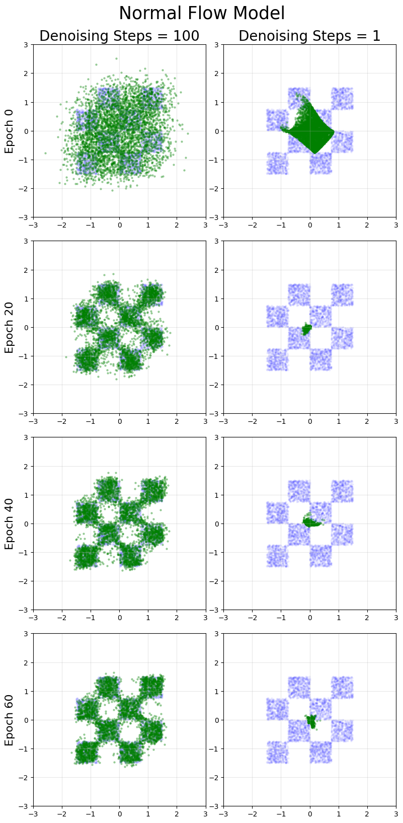
Mean Flow Example
Next, mean flow.
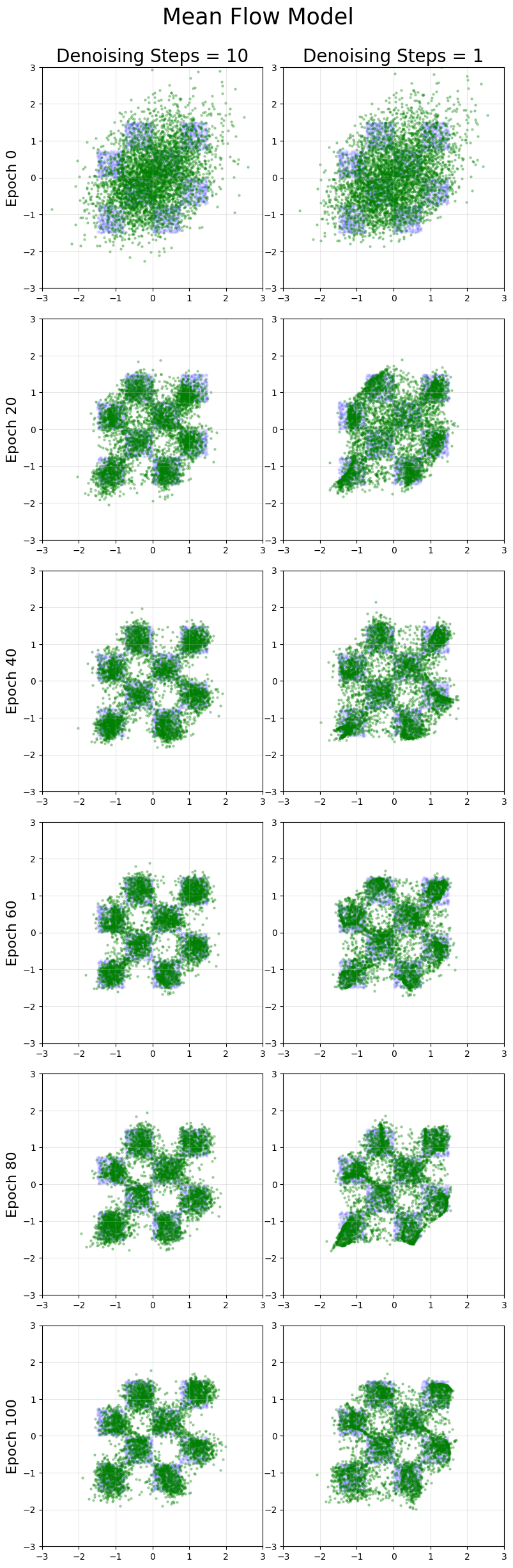
Mean flow models have good 1-step generation results (especially compared to the original flow matching models, which will never generate good 1-step generation by minimizing the loss function: see this post for details). For the checkerboard distribution, the quality of multi-step generation is slightly worse for mean flow even with more training than flow matching, which appears to be a general drawback of mean flow models.
Other 2D Distributions
Here, we compare flow matching and mean flow across a variety of distributions.
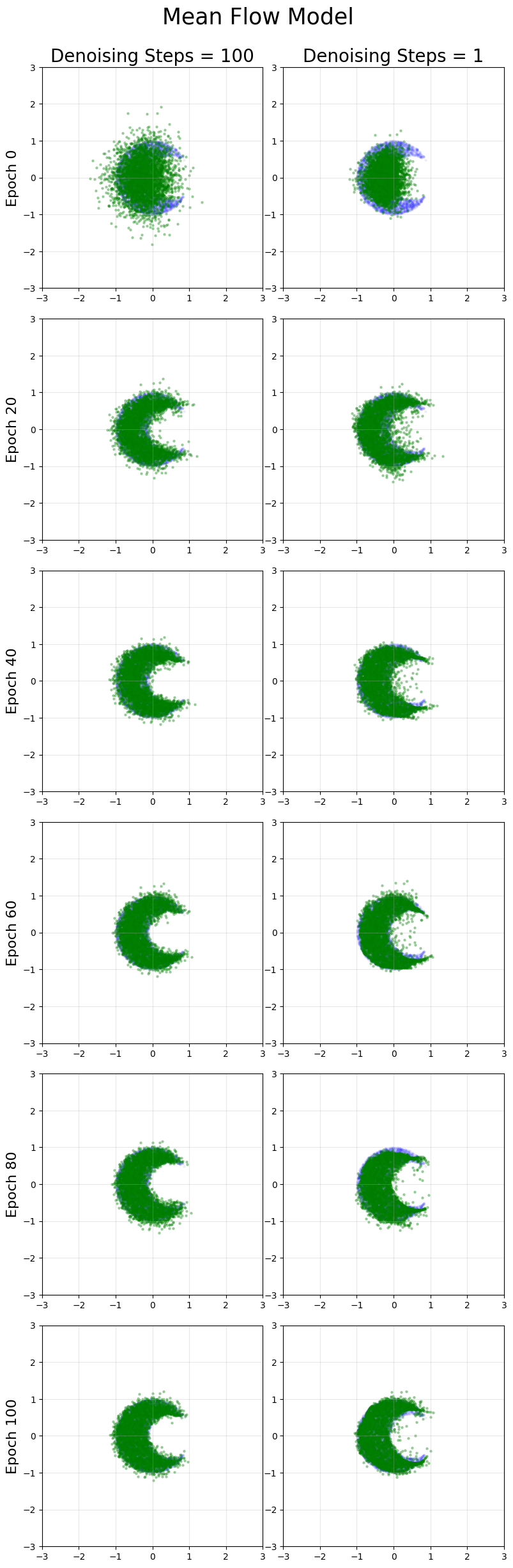
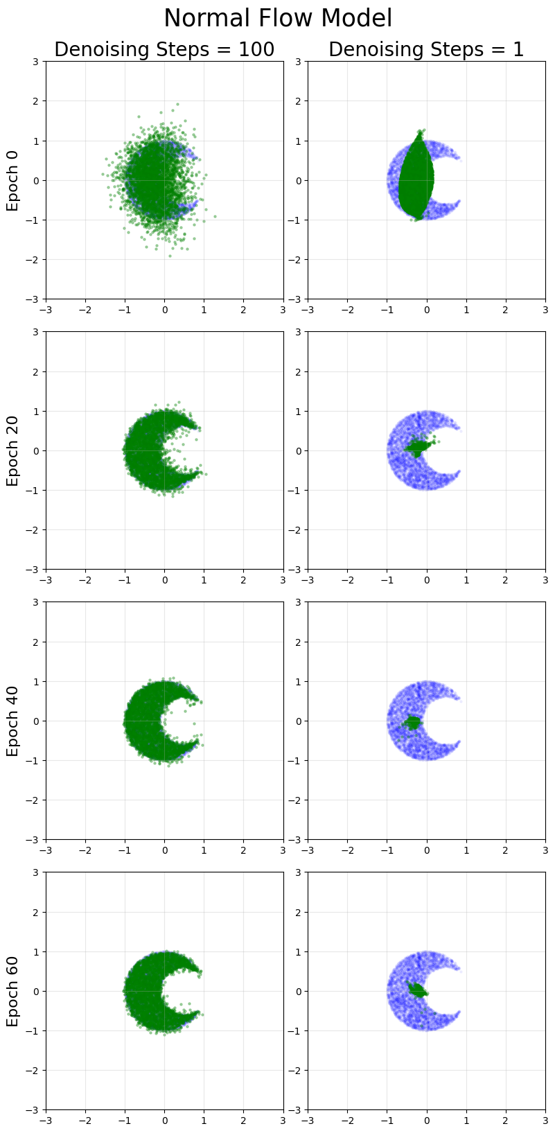
Crescent
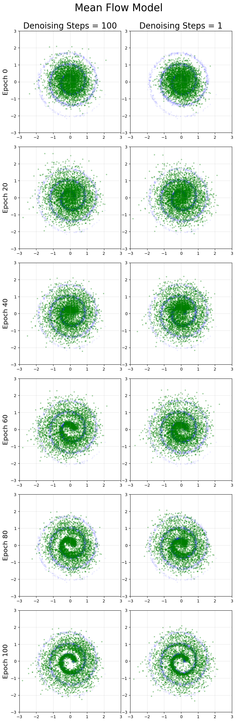
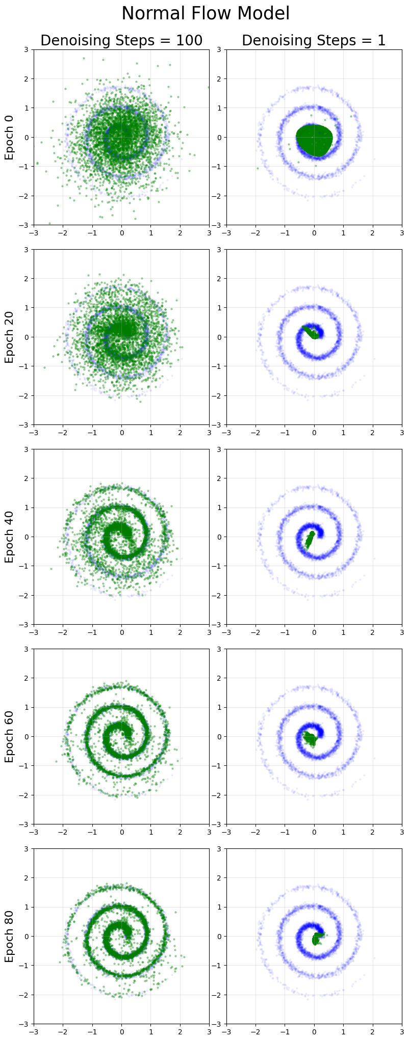
Spiral
Note this distribution is the most difficult to learn for both mean flow and flow matching.
Results
Across the 3 distributions considered here, we find excellent results for 1 step generation compared to flow matching. The multi-step generation quality is usually similar to flow matching, with the mean flow results arguably lower in quality even with more training time.
The most striking diferences were for the spiral distribution, which is the hardest for both models to learn. Flow-matching is able to achieve notably superior performance on multi-step generation with less training (not the large green regions in the mean flow that do not exist in the original spiral).
Overall Thoughts
Mean flows are an interesting method for 1 step generative modelling. Hopefully this post helps in understanding how they work, and gives a good feel for how its results as compared to standard flow matching.
For my personal (limited) experience with this framework in 2D toy settings:
- 1-step results are very impressive.
- Multi-step generation results are comparable to flow matching, but tend to be lower quality.
- Models take more epochs to train than flow matching, and the time per epoch is larger thanks to the complex loss function.
Presumably these drawbacks remain the same in more complex systems of interest. They have the ability to offer high quality single-step generation, at the cost of multi-step generation and increased training time.
If you happen to notice any mistakes or bugs, please contact me and I’ll fix it. Thanks!