How Molecular Cascades Communicate
Clarifying a common misunderstanding when applying information theory to biological data
Introduction
Information theory was originally developed in the context of optimizing electronic communications. This has resulted in much confusion when applied to the biological sciences.
This blog post is intended to clarify what information theory tells us about information transfer through a chemical cascade. It is intended as a supplement to my paper on the topic, intended for an audience new to both information theory and stochastic modelling.
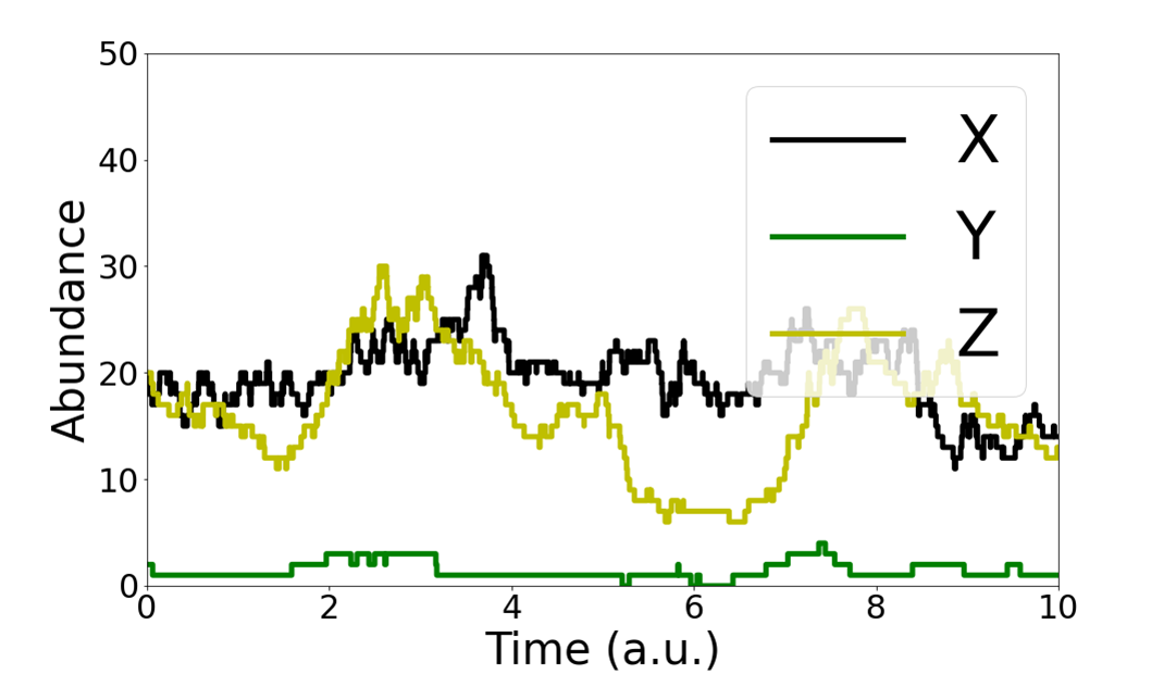
Specifically, we analyze a cascade of three species of molecules, $X \xrightarrow{} Y \xrightarrow{} Z$, where $X \xrightarrow{} Y$ denotes that the production rate of molecule $Y$ is proportional to the amount of $X$ molecules, and similarly for $Y \xrightarrow{} Z$. This represents a simple biochemical cascade.
Mathematically, the cascade is defined by the following chemical reactions
\begin{aligned} y &\xrightarrow[\phantom{y/\tau_y}]{\alpha x} y+1 &
y &\xrightarrow[\phantom{y/\tau_y}]{y/\tau_y} y-1 &
z &\xrightarrow[\phantom{z/\tau_z}]{\beta y} z+1 &
z &\xrightarrow[\phantom{z/\tau_z}]{z/\tau_z} z-1 & \end{aligned}
where the dynamics governing $x(t)$ have been left unspecified. Such cascades have been used before to model relationships between DNA, mRNA and protein.
Information Theory Basics
This section is an introduction to information theory concepts for non-experts. Those who are already familiar with information theory can skip ahead to the next section.
To communicate through our channel, we can choose an input signal $X(t)$, and the cascade will generate signals $Y(t), Z(t)$. An observer watching the behavior of $Y(t), Z(t)$ can identify characteristics of the chosen input $X(t)$ and receive information.
This idea is formalized in information theory by the mutual information between a pair of variables $X, Y$, given by the following formula
\[I(X; Y) = H(Y) - H(Y|X)\]where $ H(Y) $ denotes the entropy of $ P(Y) $, while $ H(Y | X) $ is the entropy of the conditional distribution $ P(Y | X) $. The entropy is given by
\[H(X) = \sum_x P(x) log(P(x)) .\]Entropy is an important concept in information theory, and measures spread of a distribution.
To understand the idea behind this formula, consider a communication channel that returns $Y$ given $X$. In an ideal channel, every input $X$ maps to a unique output $Y$, and thus $H(Y | X) = 0$. Then mutual information is maximized at $I(X; Y) = H(Y)$. Most channels are noisy with $H(Y | X) > 0$, lowering the information shared across this channel.
The ‘noise’ also depends on the input distribution $P(X)$. Some inputs, when sent throught he channel, result in outputs that are easier to distinguish than others.
The channel capacity is the maximum $I(X; Y)$, achieved by maximizing over all possible input distributions $P(X)$. It quantifies the maximum amount of information that can be sent through the channel.
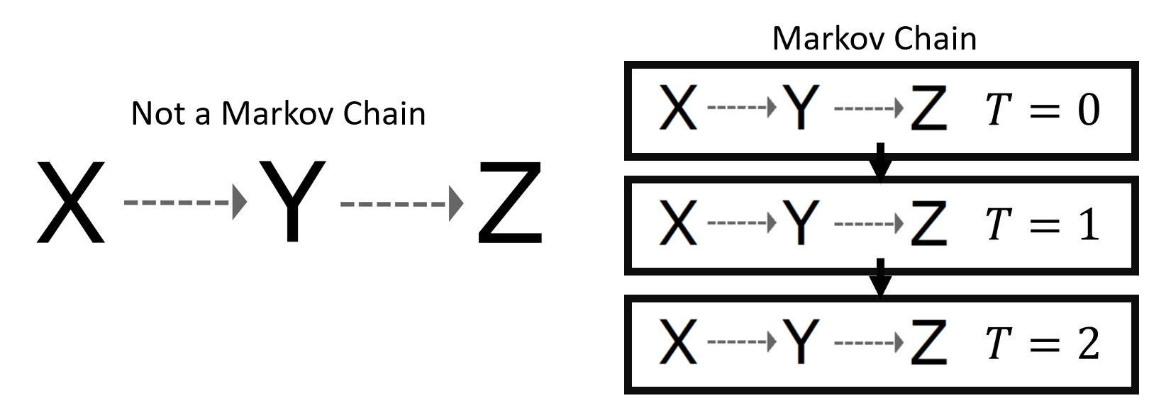
A useful property of mutual information is that it obeys the data processing inequality. The inequality states for a Markov chain $X \xrightarrow{} Y \xrightarrow{} Z$,
\[I(X; Z) \leq I(X; Y), I(Y; Z).\]Colloquially, this means mutual information between distant variables in the chain is always less than mutual information between closely related variables. The inequality is actually true as long as $P(X, Z |Y) = P(X | Y)P(Z | Y)$ (known as conditional independence ), which is true for all Markov chains $X \xrightarrow{} Y \xrightarrow{} Z$.
These properties imply we can analyze large communication networks by computing the channel capacity of individual channels. The data processing inequality tells us the channel capacity of the entire channel is given by the smallest channel capacity in the network.
Note: In the context of electrical communications, the channel capacity for a large network is achievable by transforming the data appropriately for each channel. But for a biological cascade where components are linked up directly and arbitrary transformations cannot be applied, the actual channel capacity may be much less than the individual components.
Chemical Cascades and Information
Our cascade consists of physical processes that transform inputs $X$ into outputs $Y$ from a distribution $P(Y | X)$, and is thus a channel with nonzero error rate. The input to the cascade is a time-varying signal $X(t)$, and the output is a time-varying signal $Y(t), Z(t)$.
For time-varying signals, channels are usually analyzed in terms of information transfer rates
\[R(X(t);Y(t)) = \frac{I(X(t); Y(t))}{D}\]where $D$ denotes the duration over which we use our channel. The amount of information that can be conveyed through our channel increases linearly with the duration of usage $D$. This captures the idea that we can send arbitrarily large amounts of information through poor communication channels given enough time.
To transfer information in our cascade, select an input time trace $X(t)$ of duration $D$. The physical processes of our channel convert the input into output time traces $Y(t), Z(t)$ with associated probabilities $P(Y(t) | X(t)), P(Z(t) | X(t))$. Channel quality is measured by rates $R(X(t);Y(t)), R(X(t);Z(t))$.
For our chemical cascade, $P(Z(t) | Y(t), X(t)) = P(Z(t) | Y(t))$ since the time trace of $Z(t)$ only depends on $X(t)$ through how it affects $X(t)$ by definition, so the data processing inequality holds for the rates.
Distinct Channels In Our Cascade
To determine information rates, note our cascade consists of four physical processes that generate new time traces given the preceding result as input.
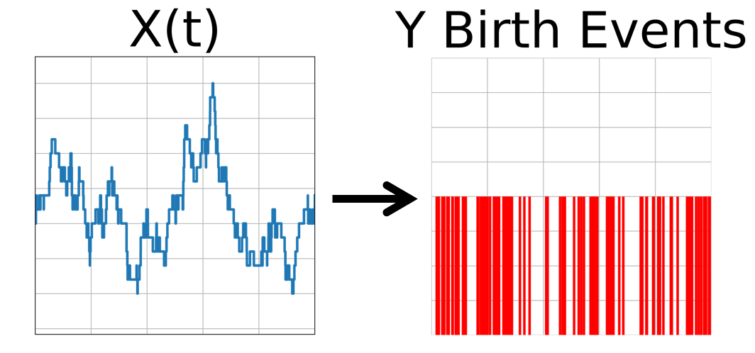
The first process is
\begin{aligned} y \xrightarrow{\alpha x} y+1 \end{aligned}
which from input time trace $X(t)$, generates a time trace $Y_{birth}(t)$ that tracks all the $y$ molecule production events that occur over the interval of usage $D$.
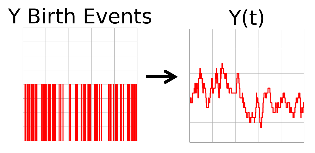
The second process is
\begin{aligned} y \xrightarrow{y/\tau_y} y-1 \end{aligned}
which uses $Y_{birth}(t)$ and an initial number of $y$ molecules, and generates the time trace $Y(t)$ using the random degradation of y molecules.
The other two physical processes are
\begin{aligned} z &\xrightarrow[\phantom{z/\tau_z}]{\beta y} z+1 &
z &\xrightarrow[\phantom{z/\tau_z}]{z/\tau_z} z-1 & \end{aligned}
which generate $Z_{birth}(t)$ from $Y(t)$, and then $Z(t)$ using $Z_{birth}(t)$ births and an initial $Z(t = 0)$ value of molecules.
Capacity Of The Distinct Channels
Our cascade consists of two types of processes, production events and degradation events. Here we discuss the capacity of these processes.
The first process
\begin{aligned} y \xrightarrow{\alpha x} y+1 \end{aligned}
corresponds to a well studied channel in the optical communications literature, known as the direct detection photon channel. Several results for the channel capacity are known under different constraints for $\alpha x$, which we briefly include here.
Channel Capacity Under Different Input Constraints
These results are taken from this supplement. If $\alpha x \leq A_{max}$, then it is known that the capacity is
\[C = A_{max} / e\]If the mean $\alpha \langle x \rangle$ is also constrained, then the capacity becomes
\[C = \alpha \langle x \rangle \log \left( \frac{A_{max}}{\alpha \langle x \rangle} \right)\]These capacities are realized by sending in $x(t)$ that oscillates between 0 and $A_{max}$ instantaneously. This is highly nonphysical for biological systems.
The first capacity can be proven by breaking up the usage of the channel for duration $D$ into using the channel $N$ times each for a duration $D/N$. For large $N$ each use of the channel is equivalent to a Z channel with an error rate proportional to $N$, and taking the limit $N \xrightarrow{} \infty$ yields the capacity above. The optimal input time trace follows from the optimal inputs to the Z channel.
Another constraint has been derived when the first two moments of the input signal are fixed, yielding
\[C = \alpha \langle x \rangle \log \left(1 + \frac{\sigma^2_f}{\langle x \rangle^2}\right) \leq \frac{\sigma^2_f}{\langle x \rangle}\]For the second process
\begin{aligned} y \xrightarrow{y/\tau_y} y-1 \end{aligned}
which uses $Y_{birth}(t)$ and an initial number of molecules to generate $Y(t)$, observe $Y_{birth}(t)$ can always be accurately inferred from $Y(t)$, since molecular production events are easily detectable. Therefore the channel capacity of this process is always the entropy of the input $Y_{birth}$.
Thus the channel capacity of $X \rightarrow Y$ is the channel capacity of the production reaction, which has been studied before for various constraints.
Conditional independence between $X(t), Z(t) | Y(t)$ thus implies the channel capacity of the full cascade is
\[C_{X\rightarrow Y \rightarrow Z} = \textbf{min}(C_{X\rightarrow Y }, C_{Y\rightarrow Z })\]Existing Biological Experimental Data
In practice, it is difficult to measure time traces of multiple molecules inside of living cells simultaneously. Furthermore, the mutual information discussed above applies to distributions of time traces, which is hard to estimate from experimental data (any specific time trace has near zero probability).
However, it is possible to measure the abundances of multiple molecules in recently deceased cells. This can be done on large numbers of cells to obtain joint probability distributions of instantaneous molecular abundances, illustrated in the following figure. This data can be analyzed to infer properties of the underlying relationships.
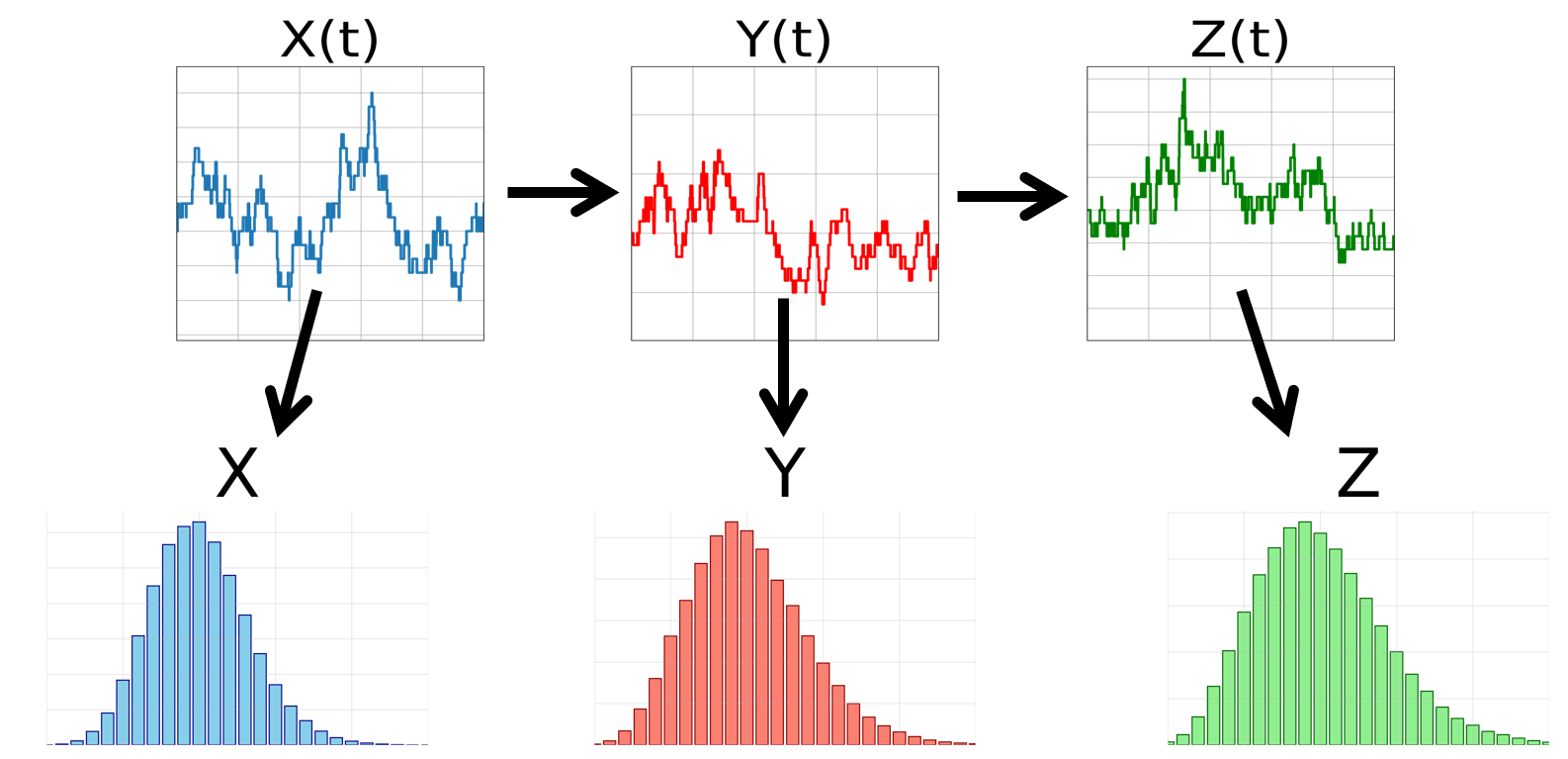
Note instantaneous joint distributions do not obey the same properties as the underlying joint distributions of time traces. Instead, they are derived from the time trace distribution through randomly sampling the time traces at the same time.
Such joint distributions still contain useful information theoretic properties. Consider the probability distribution of time traces $P(X(t))$. From this we derive both the sequence of birth events $Y_{birth}$ (and thus the time trace $Y(t)$), and the probability distribution of instantaneous $X$ values. Thus we find $X, Y(t)$ are conditionally independent of each other given $X(t)$.
However, the link between the different instantaneous distributions only arises from averaging the related time traces. The different instantaneous values of $X, Y, Z$ do not form a proper communication channel $X \rightarrow Y \rightarrow Z$, and thus $X, Z$ are not conditionally independent of each other given $Y$ - they become independent only when conditioned on $X(t), Y(t)$ or $Z(t)$.
Violations Of The “Data-Processing Inequality”
A consequence of analyzing the static distributions from experiments is that the data processing inequality is no longer true. This is because the variables $X, Y, Z$ do not form a channel.
This allows for biological cascades to generate distributions in experiments that violate the inequality. This was covered in detail in the paper, where mathematics and numerical simulations have been used to explore the regime of parameter space for which these inequalities break down. This is illustrated in the following figure, where simulating a cascade for a variety of parameters reveals regions of parameter space for which the mutual information $I(X; Z) > I(X; Y)$ (blue region).
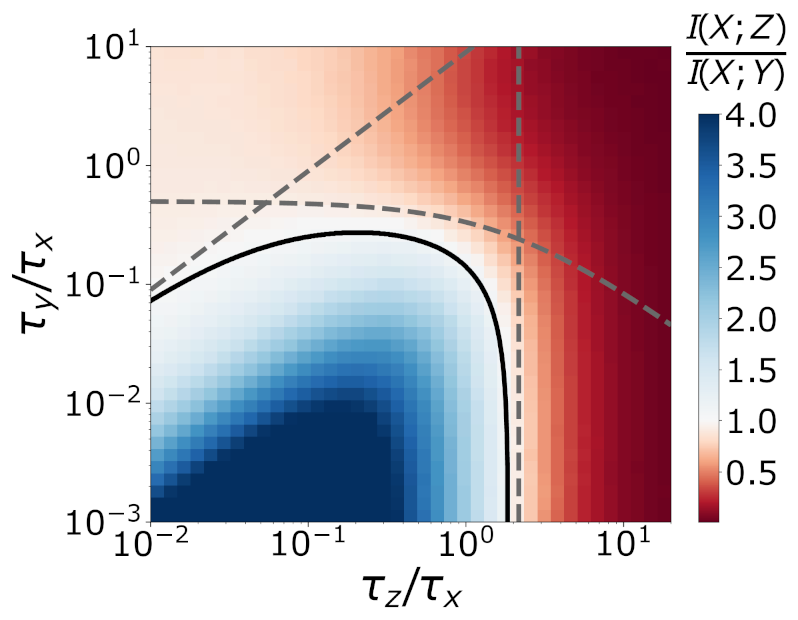
For a simple intuitive explanation of how this can occur, consider the problem of estimating the instantaneous value of $X$. Suppose the abundance of $Y$ is very small, such that low copy number noise is very significant. Then for any value of $X$, there is a large variety of $Y$ values, and it is difficult to estimate $X$ from $Y$.
Suppose $Y$ molecules have a very short lifetime compared to $X, Z$ molecules. Then the abundance $Y$ will oscillate very quickly. $Z$ molecules, which are made proportional to the amount of $Y$ molecules, will experience rapid fluctuations in their birth rate. But the $Z$ abundance is related to the number of $Z$ molecules made over the average lifetime of a $Z$ molecule, and thus does not vary much if the $Z$ lifetime is large compared to the $Y$ molecule lifetime.
In this way, we can accurately estimate the current value of $X$ by looking at the $Z$ abundance, since $Z$ time-averages out the large amount of $Y$ noise. This idea of estimation is closely linked with the mutual information (which represents the reduction in uncertainty about the value of $X$).
On Actual Inequalities
In this post, we’ve seen how the data processing inequality applies to chemical cascades only when considering the distribution of time traces.
The often experimentally measured instantaneous distributions of molecules however, do not obey these inequalities because they do not form a Markov Chain with respect to each other, and there exist parameter regimes where even simple cascades can display apparent ‘violations’.
This observation prompts a deeper question:
Can we derive new inequalities that apply to these experimentally accessible (static) distributions?
Surprisingly, yes—but with caveats.
While we saw that $Y$ can accumulate arbitrary information from $X$ over time, accurate information about the current state of $X$ is different, as older information becomes irrelevant. There is a competition between:
- The rate at which $Y$ learns about $X$ (governed by the production reaction)
- The rate at which $X$’s state changes (governed by X’s dynamics)
Unlike the DPI, these new inequalities are dependent on the dynamics of the system involved and do not generalize. Furthermore, they’re mathematically difficult to derive and work with.
I’ll discuss more on this topic in more detail in a future blog post, on “Inequalities for Static Distributions in Biochemical Cascades”.