Do Conservative PINNs Train Faster In High Dimensions?
Alternatively, how strong is a conservative vector field as an inductive bias?
The code and experimental results for this post are available on github.
Introduction
Hamiltonian Neural Networks are a type of physics informed neural network (PINN). Their predictions result in more physically accurate simulations since they conserve energy, making them attractive for physics purposes.
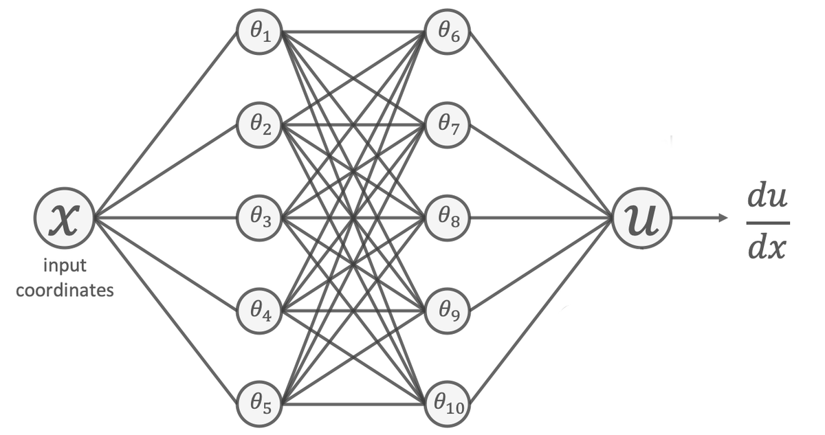
They work by using coordinates $(x_1, x_2, …, x_n)$ to predict a scalar $U(x_1, …, x_n)$, and then automatic differentiation computes the gradients $\left(\frac{dU}{dx_1}, …, \frac{dU}{dx_n}\right)$ which are compared to training data. This differential structure guarantees its predictions will conserve energy, whereas a network that predict gradients directly generally does not conserve energy.
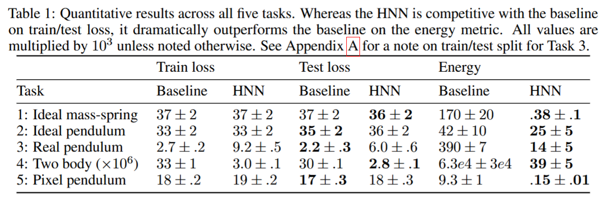
In the original paper, the authors mentioned there were negligible differences in the test/train losses for a baseline NN and the Hamiltonian NN. It is only when the networks are used for a long time that the differences in energy conservation become apparent.
But is that really true?
Training Speed
In the original paper, experiments were done for mostly low-dimensional problems. The only case that the Hamiltonian NN showed significant improvement was also the only one with more than 2 system coordinates (the 2-body problem has 4 spatial and momentum coordinates, for a total of 8 coordinates).
Hamiltonian NNs work by learning a single scalar function $U$ instead of $d$ separate gradient components. In theory, this suggests we should observe more significant speedups when the dimension of the problem is increased, which could explain the results in the previous paper.
In practice, automatic differentiation could be too numerically unstable, or the scaling is too minor: it’s well known neural networks scale really well with high dimensions (growing polynomially instead of exponentially) so the effect of this differential structure may be too minor.
In this blog post, we’ll test whether higher dimensions reveal clearer advantages in training speed through a toy conservative vector field problem.
Experiment Design
Our question: Does a network with the inductive bias of a conservative vector field built in via the gradient procedure in Hamiltonian Neural Networks train faster than a baseline network as dimensionality increases?
The Toy Problem
We construct a $d$-dimensional problem with inputs being coordinates $\vec{x} = (x_1, …, x_d)$ in $[-1,1]^d$, and a target output vector field $f(\vec{x})$ derived from a sum of Gaussians:
\[f(\vec{x}) = \sum_{i=1}^N -a_N \exp\left(-\frac{||\vec{x} - \vec{c}_N||^2}{\sigma_N^2}\right) (\vec{x} - \vec{c}_N)\]Here $\vec{c}_N$ are randomly located Gaussian centers with amplitudes and widths $a_N, \sigma_N$. This vector field is conservative, since $f(\vec{x})$ is the gradient of a scalar sum of Gaussians.
Network Architectures
We compare two approaches:
-
Baseline Network:
Directly predicts all $d$ output components $(y_1, …, y_d)$. -
Conservative Network:
Predicts a scalar potential $U(\vec{x})$, with gradients $\left(\frac{dU}{dx_1}, …, \frac{dU}{dx_n}\right) = \vec{y}$ computed via automatic differentiation.
Both use identical hidden-layer architectures, differing only in input/output dimensions. We analyze how the train and test losses behave as we scale the dimension of the problem.
Scaling with Dimension
Fixed Parameters
-
Network Size: Hidden layers are fixed; Input and output(baseline network only) layers grow with $d$.
-
Test and Training Points: Fixed at $t_{test}, t_{train} = 10^4$. This reflects real-life high-dimensional problems, where training and test data is limited and does not grow with dimension.
-
Gaussian Amplitudes: All amplitudes are equal, fixed at 1.
-
Gaussian Variances: Variances are chosen uniformly from $[0.5, 1.0]$. This spread was chosen to make sure the different centers have different variances, and the variances are not so large as to cover all of space, nor so small as to make dense coverage of the space impossible without an exorbitant amount of points.
Three Experimental Regimes
We test three approaches for the scaling underlying vector field with dimension, determined solely by the number of Gaussian centers.
Constant Density: As the dimension increases, the number of Gaussian points increase accordingly, via the following scaling law
\[N \propto \frac{V_{\text{cube}}}{\langle V_{\text{Gaussian}} \rangle} = \frac{2^d}{\langle \sigma^d \rangle} \cdot \frac{\Gamma\left(\frac{d}{2} + 1\right)}{\pi^{d/2}}\]which approximately ensures each Gaussian can have 1 $\sigma$ of space around itself without overlaps. Note that due to random center generation, they will not end up evenly spread.
Fixed N = 15: As the dimension increases, the number of Gaussian points stays fixed at $N = 15$. This number was chosen arbitrarily.
Fixed N = 2: The number of Gaussian points stays fixed at $N = 2$. This was chosen to be simpler than the previous case, to observe how the problem difficulty affects the results.
These three regimes span a wide variety of cases, from a problem whose complexity scales with dimension to a simple problem defined by the location of two points in $d$-dimensional space, and their corresponding variances.
Hypothesis
The conservative constraint should become more useful in high dimensions, since the baseline network must learn d independent functions, but the conservative network learns just one scalar potential.
Therefore the conservative network should have lower train and test losses per epoch than the baseline network as the dimension of the problem is increased, regardless of the experimental regime.
Results
We tested networks across a variety of dimensions for the three experiments. For each dimension, three architectures were used:
| Network Configuration | Hidden Layers |
|---|---|
| Small | [64, 64, 64] |
| Medium | [128, 128, 128] |
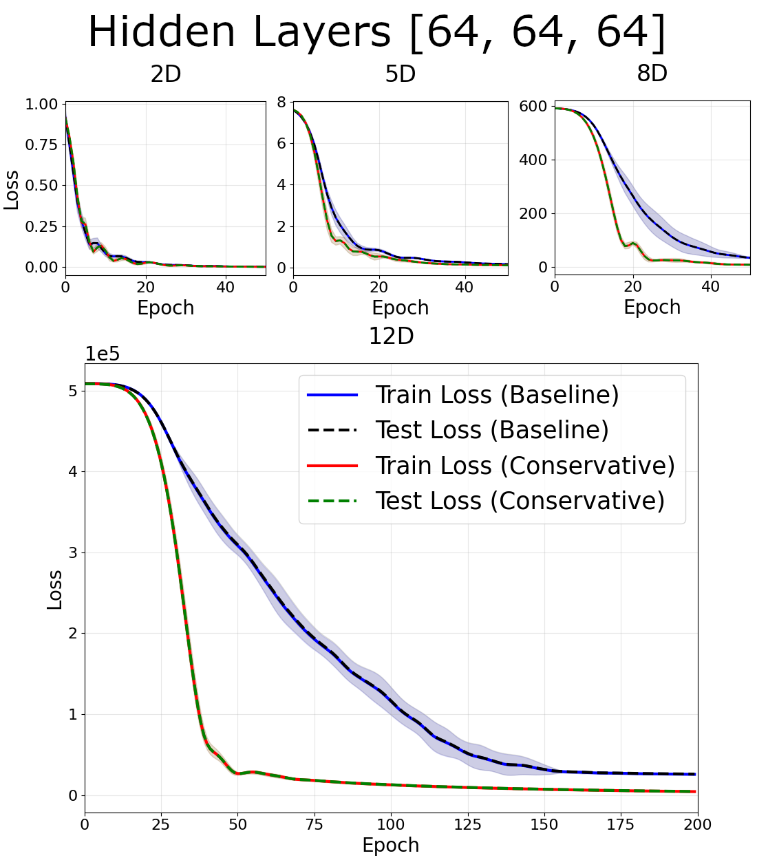
| Large | [256, 256, 256] |
Each architecture was trained with 10 different weight initializations each on 10 different randomly generated datasets to ensure reported results are not artifacts of peculiar initializations. All data (Gaussian parameters as well as training and test points) were generated with fixed random seeds for reproducibility.
The train and test losses behaved almost identically for all architectures and datasets. All reported results occured regardless of weight initializations or dataset generation.
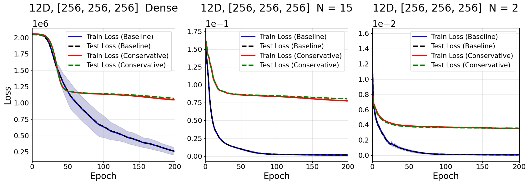
Dense Gaussians
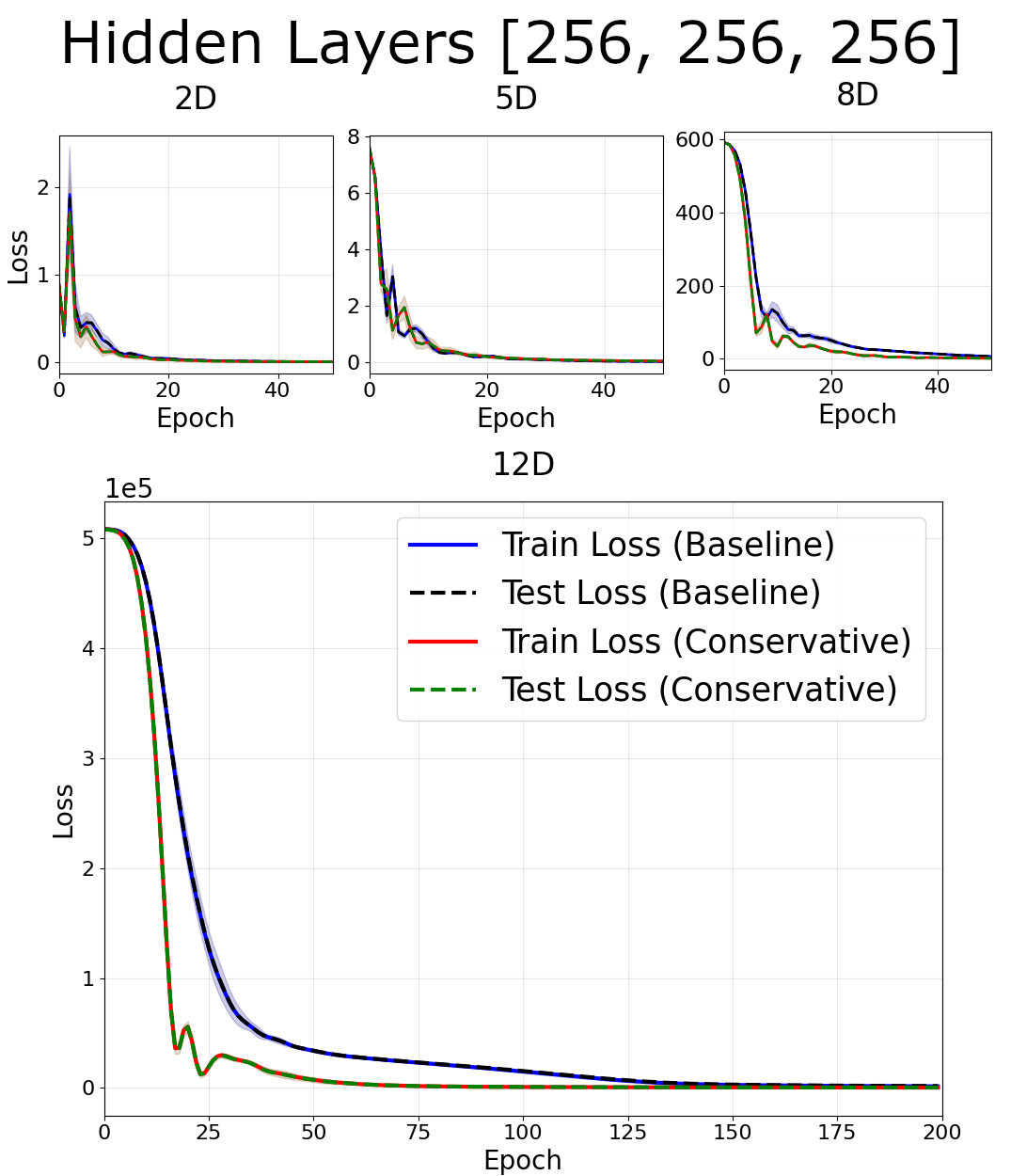
In the dense case, little differences were observed between losses at $d < 8$. At $d \geq 8$, there were notable decreases in the train/test loss for conservative networks. These trends occured in all network architectures, with the most significant effects for smaller networks.
N = 15 Gaussians
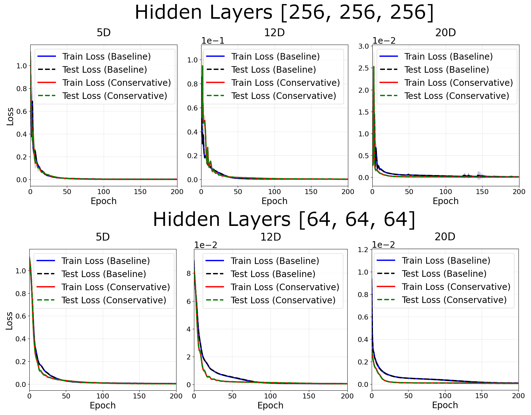
For fixed center number $N = 15$, there was little difference between between losses at small dimension, and notably smaller loss at higher dimensions. For fixed center number it is easy to increase the dimension of the problem, so we test up to $d = 20$. Smaller networks enjoy greater advantages from the conservative bias.
Note the advantages of a conservative network are much smaller for the fixed center number than in the dense case.
N = 2 Gaussians
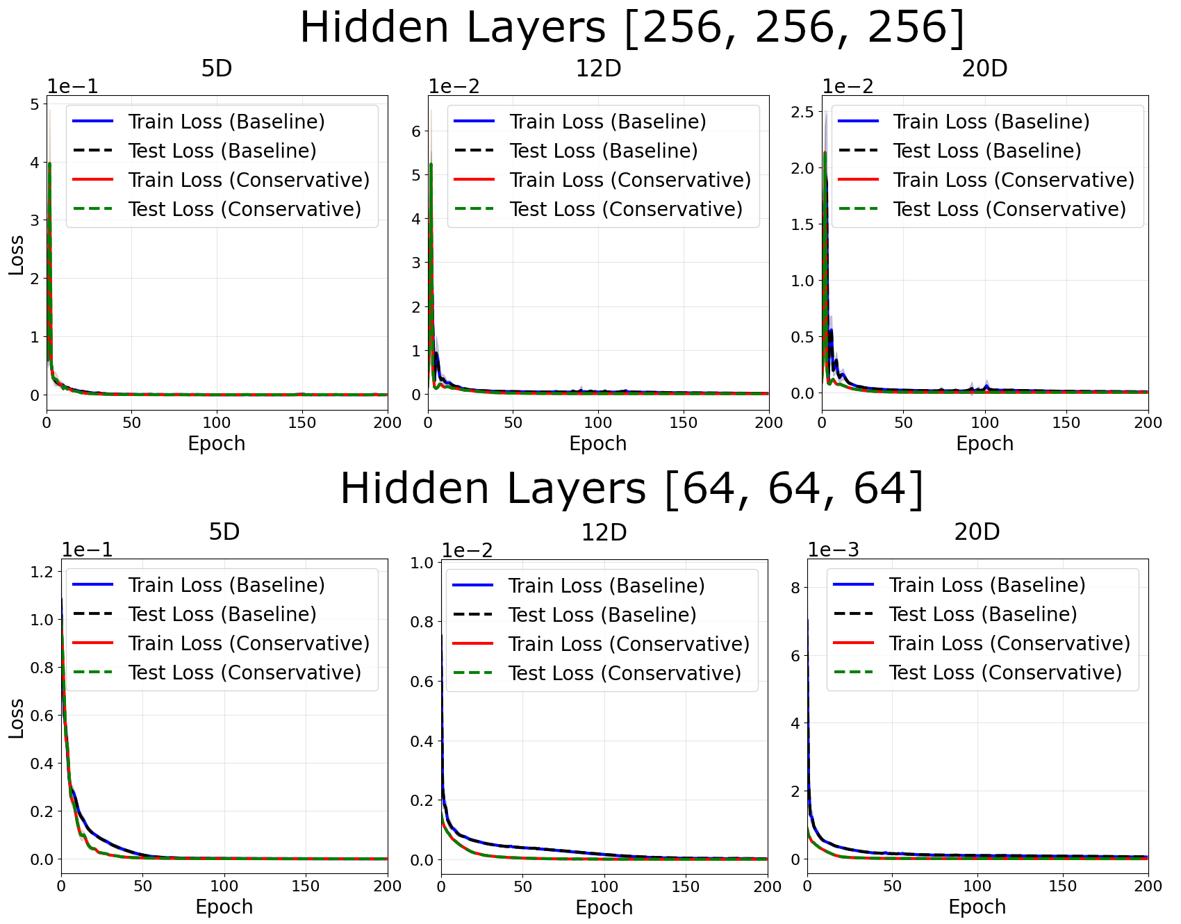
For $N= 2$ Gaussians, the loss again only notably decreases at high dimensions, with effects more severe in smaller networks.
Control Experiment: Non-Conservative Field
To verify results arise from our conservative inductive bias, we test our networks on a non-conservative field. This field was achieved by multiplying our conservative vector field outputs by a fixed matrix of constant coefficients.
The performance of conservative networks degraded significantly here. showing that our observed improvements in training speed occur because our conservative networks are well-suited to predicting conservative vector fields.
More data for other dimensions, other initializations of datasets and the intermediate architecture size can be found on the github repo.
Discussion
Hamiltonian networks contain inductive biases inspired from physics, and their advantages in accurately simulating physical systems are well established.
This work instead examined whether networks with a built-in conservation law (such as Hamiltonian NNs) improved training speed. The results showed these networks have smaller training and test loss for a given epoch when the dimension of the problem is very high. This is consistent with results from the original, where the only system to show improvements in training and test loss was the two body problem, which has 8 system coordinates (4 spatial coordinates and 4 velocity coordinates). However, the reduction in loss was fairly minor, with baseline networks almost always achieving lower loss when given x3 the number of epochs.
This aligns with the theoretical expectation that learning a scalar potential should be simpler than a $d$ diemsnional vector field. Unfortunately, there is no evidence of a general scaling law for the training speedup of a conservative network, as the speedup effects are dependent on the architecture and do not appear to generalize. See example figures on the ratio of test losses in the github repo.
In this comparison I’ve neglected the additional compute time cost of the conservative network. The conservative network generates a scalar, and automatic differentiation is needed for gradients. Automatic differentiation is also used in computing the loss, and constitutes a significant amount of time in training networks.
In our experiments, this makes our conservative networks take roughly twice as long per epoch. Plotting the compute time instead of epoch number, we find very minor gains in training performance assuming they do not disappear entirely.
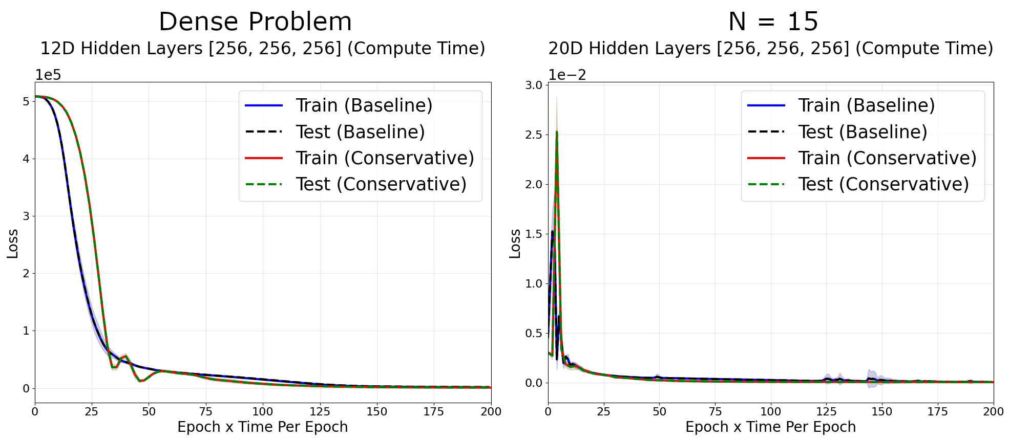
Note: It’s not clear to me that this slowdown is fundamental and can’t be sped up with clever gradient accumulation, so this problem may be fixable.
These findings suggest the gains by a conservative architecture in speeding up training speeds is relatively modest, especially when training large networks. The advantages are larger for smaller networks.
Closing Thoughts
Although the original paper on Hamiltonian Neural Networks focused on many simple low-dimensional problems, many interesting problems in physics are very high dimensional. Since the conservative vector field bias built-in Hamiltonian Neural Networks intrinsically scales with dimension, I thought they could turn out to be extemely useful if they scaled very well.
For example, convolutional neural networks make use of translational invariance and demonstrate large advantages in tasks with such symmetries (eg, most computer vision tasks). While such speedups would be unlikely for Hamiltonian Neural Networks (the conservative constraint seems much weaker than translational invariance), it does leave some hope that they might scale well in a meaningful way.
Sadly, our results show that while speed benefits appear in higher dimensions, they are relatively modest. As an (unproven) explanation, it seems the natural ability of neural networks to perform extremely well in high dimensions suppresses the modest dimensional scaling of a conservative vector field. Furthermore, difficulties with multiple uses of automatic differentiation make the modest benefits in training speed fairly negligible, barring the most extreme cases.
If you found the contents of this blog post useful, or have any questions, please feel free to leave a comment.